operations management
Chapter 13 - Inventory Management
Chapter 13
Inventory Management
Teaching NotesThis is a fairly long and important chapter. Important points are:
1. Good inventory management is important for successful organizations.
2. The key issues are when to order and how much to order.
3. Because all items are not of equal importance, it is necessary to establish a classification system for allocating resources for inventory control.
4. EOQ models answer the question of how much to order. Variations of the basic EOQ model include the quantity discount model and the economic run size model.
5. EOQ models tend to be rather robust: even though one or more of the parameters may be only roughly correct, the model can yield a total cost that is close to the actual minimum.
6. ROP models are used to answer the question of when to order. Different models are used, depending on whether demand, lead time, or both are variable.
7. Other models described are the fixed interval model and the single period model in the supplement.
8. All of the models in this chapter pertain to independent demand.
The Single-Period Model is used to handle ordering of perishables (such as fresh fruits and vegetables, seafood, and cut flowers) as well as items that have a limited useful life (such as newspapers and magazines). Analysis of single-period situations generally focuses on two costs: shortage and excess. Shortage costs may include a charge for loss of customer goodwill as well as the opportunity cost of lost sales or unrealized profit per unit. Excess cost pertains to items left over at the end of the period and is the difference between purchase cost and salvage value. There may be costs associated with disposing of excess items which would make the salvage value negative and hence increase the excess cost per unit.
1. Inventories are held (1) to take advantage of price discounts, (2) to take advantage of economic lot sizes, (3) to provide a certain level of customer service, and (4) because production requires some in-process inventory.
2. Effective inventory management requires (1) cost information, information on demand and lead time (amounts and variabilities), an accounting system, and a priority system (e.g., A-B-C).
3. Carrying or holding costs include interest, security, warehousing, obsolescence, and so on. Procurement costs relate to determining how much is needed, vendor analysis, inspection of receipts and movement to temporary storage, and typing up invoices. Shortage costs refer to opportunity costs incurred through failure to make a sale due to lack of inventory. Excess costs refer to having too much inventory on hand.
4. The RFID (Radio Frequency Identification) chip tags are beginning to be used with consumer products and they contain bits of data, such as product serial number. Scanners will automatically read the information on an RFID chip into a database, so the companies can keep track of sales and inventory. Keeping track of inventory will enable suppliers to keep track of trends and react to market changes. In addition, RFID chips will assist in increasing the speed of communication on a supply chain. The information between parties will travel faster, which will improve the responsiveness of buyers and ordering information on the supply chain. The risk of using RFID chip tags stems from privacy concerns. It is feared that computer pirates will figure out security controls and be able to scan shoppers’ merchandise and determine what they have bought. In order to avoid this risk, companies are considering turning of RFID tags once the items are purchased.
5. It may be inappropriate to compare the inventory turnover ratios of companies in different industries because the production process, requirements and the length of production run varies across different industries. The shorter the production time, the less the need for inventory.
In addition, the material delivery lead times may vary between different industries. The higher the variability of lead time and the longer the lead time, the greater the need for inventory. As supplier reliability increases, the need for inventory decreases. The industries with higher forecast accuracies have less of a need for inventories.
6. a. Only one product is involved.
b. Annual demand requirements are known.
c. Demand is spread evenly throughout the year so that the demand rate is reasonably constant.
d. Lead time does not vary.
e. Each order is received in a single delivery.
f. There are no quantity discounts
7. The total cost curve is relatively flat in the vicinity of the EOQ, so that there is a “zone” of values of order quantity for which the total cost is close to its minimum. The fact that the EOQ calculation involves taking a square root lessens the impact of estimation errors. Also, errors may cancel each other out.
8. As the carrying cost increases, holding inventory becomes more expensive. Therefore, in order to avoid higher inventory carrying costs, the company will order more frequently in smaller quantities because ordering smaller quantities will lead to carrying less inventory.
9. Safety stock is inventory held in excess of expected demand to reduce the risk of stockout presented by variability in either lead time or demand rates.
10. Safety stock is large when large variations in lead time and/or usage are present. Conversely, small variations in usage or lead time require small safety stock. Safety stock is zero when usage and lead time are constant, or when the service level is 50 percent (and hence, z = 0).
11. Service level can be defined in a number of ways. The text focuses mainly on “the probability that demand will not exceed the amount on hand.” Other definitions relate to the percentage of cycles per year without a stockout, or the percentage of annual demand satisfied from inventory. (This last definition often tends to confuse students in my experience.)
Increasing the service level requires increasing the amount of safety stock.
12. The A-B-C approach refers to the classification of items stocked according to some measure of importance (e.g., cost, cost-volume, criticalness, cost of stockout) and allocating control efforts on that basis.
13. In effect, this situation is a “quantity discount” case with a time dimension. Hence, buying larger quantities will result in lower annual purchase costs, lower ordering costs (fewer orders), but increased carrying costs. Since it is unlikely that the compressor supplier announces price increases far in advance, the purchasing agent will have to develop a forecast of future price increases to use in determining order size. Unlike the standard discount approach, the agent may opt to use trial and error to determine the best order size, taking into account the three costs (carrying, ordering and purchasing). In any event, it is reasonable to expect that a larger order size would be more appropriate; although obsolescence may also be a factor.
14. Annual carrying costs are determined by average inventory. Hence, a decrease in average inventory is desirable, if possible. Average inventory is Qo/2, and Qo decreases (run size model) if setup cost, S, decreases.
15. The Single-Period Model is used when inventory items have a limited useful life (i.e., items are not carried over from one period to the next).
16. Yes. When excess costs are high and shortage costs are low, the optimum stocking level is less than expected demand.
17. A company can reduce the need for inventories by:
using standardized parts
improved forecasting of demand
using preventive maintenance on equipment and machines
reducing supplier delivery lead times and delivery reliability
utilizing reliable suppliers and improving the relationships in the supply chain
restructuring the supply chain so that the supplier holds the inventory
reducing production lead time by using more efficient manufacturing methods
developing simpler product designs with fewer parts.
1. a. If we buy additional amounts of a particular good to take advantage of quantity discounts, then we will save money on a per unit purchasing cost of the item. We will also save on ordering cost because since we bought a larger quantity, we will not have to order this item as frequently. However, as a result of ordering larger quantity, we will have to carry larger inventory in stock, which in turn will result in an increase in inventory holding cost.
b. If we treat holding cost as a percentage of the unit price, as the unit price increases, so will the holding cost, and as a result, if we are using the EOQ approach, we will have to place a smaller order, resulting in a lesser inventory. On the other hand, if we use a constant amount of a holding cost, the inventory decisions will not be affected by the changes in unit cost (price) of the item.
c. Conducting a cycle count once a quarter instead of once a year will result in more frequent counting, which will result in an increase in labor and overhead costs. However, the more frequent counting would also lead to less errors in inventory accuracy and more timely detection of errors, which in turn would lead to timely deliveries to customers, less work in process inventory, more efficient operations, improved customer service, and assurance of material availability.
2. In making inventory decisions involving holding costs, setting inventory levels and deciding on quantity discount purchases, the materials manager, plant manager, production planning and control manager, the purchasing manager, and in some cases the planners who work in production planning and control or purchasing departments should be involved. The level and the nature of involvement will depend on the organizational structure of the company and the type of product being manufactured or purchased.
3. The technology has had a tremendous impact on inventory management. The utilization of bar coding has not only reduced the cost of taking physical inventory but also enabled real time updating of inventory records. The satellite control systems available in trucks and automobiles has enabled companies to determine and track the location of in-transit inventory.
1. Including a wider range of foods provide fast food companies with a competitive edge in terms of improving customer satisfaction and service. However, it has also complicated the operational function of the company. Expansion of menu offerings can create problems for inventory management because there are more ingredients and inventory items to order and to control the levels of inventory. This means higher labor costs in terms of placing orders, increased storage facility needs and increased need for coordinating the shipments from the supplier so that deliveries can be at low cost and efficient. Increasing the variety of items on the menu will also cause problems with forecasting. Since we have more items on the menu, it is likely that the demand for current menu items will decrease. The forecasts for all items will need to be revised. If we are not able to estimate this possible decrease, then the forecasting problem will result in excess or insufficient inventory levels.
2. a. How important is the item? For example, does it relate to a holiday or other important event,
such as graduation cards?
b. Are comparable substitutes readily available?
c. What competitor alternatives are available to customers?
d. Is this an occasional occurrence, or indicative of a larger, perhaps ongoing, problem?
3. Among considerations are:
How many stamps does he now have? Does he know how many he has? If so, how many?
What is his usage rate or current need for stamps?
What else does he need the cash for today?
Can he get more money at a bank or ATM?
How long will it be before he will return to the post office?
Will the post office be closed for a holiday or a Sunday?
Can he buy stamps elsewhere in case he runs low?
How convenient is it for him to visit the post office?
Can he purchase “forever stamps” and temporarily avoid a price increase?
4. Student answers will vary.
Memo Writing Exercises1. Cost of carrying inventory must be weighted against the following costs:
cost of shortages (finished goods inventory)
cost of failures (work-in-process inventory)
cost of supplier reliability
cost of ordering
cost of setups
cost of quantity discounts
cost of smoothing production for seasonal products.
2. The possible advantages of using a single supplier include:
obtaining a discount due to additional volume purchased from the supplier
building trust and working with the supplier so that the material will be delivered in a timely fashion to avoid stockouts and excess inventory.
The possible advantages of using multiple suppliers include:
the adverse effect of tardiness will be felt much less when there are multiple sources for the materials.
The main advantage of using the fixed order interval model is the reduction in ordering cost because orders for different parts are aggregated during the order interval.
The main disadvantage of using the fixed order interval model is that the company faces the risk of experiencing shortages during the fixed interval.
In this particular situation, the advantages of using a single supplier may be offset by using the fixed order interval model.
Solutions
| 1. a. | | Item | Usage | Unit Cost | Usage x Unit Cost | Category |
| | | 4021 | 90 | $1,400 | $126,000 | A |
| | | 9402 | 300 | 12 | 3,600 | C |
| | | 4066 | 30 | 700 | 21,000 | B |
| | | 6500 | 150 | 20 | 3,000 | C |
| | | 9280 | 10 | 1,020 | 10,200 | C |
| | | 4050 | 80 | 140 | 11,200 | C |
| | | 6850 | 2,000 | 10 | 20,000 | B |
| | | 3010 | 400 | 20 | 8,000 | C |
| | | 4400 | 5,000 | 5 | 25,000 | B |
In descending order:
| | | Item | | Usage x Cost | | Category |
| | | 4021 | | $126,000 | | A |
| | | | | | | |
| | | 4400 | | 25,000 | | B |
| | | 4066 | | 21,000 | | B |
| | | 6850 | | 20,000 | | B |
| | | | | | | |
| | | 4050 | | 11,200 | | C |
| | | 9280 | | 10,200 | | C |
| | | 3010 | | 8,000 | | C |
| | | 9402 | | 3,600 | | C |
| | | 6500 | | 3,000 | | |
| | | | | 228,000 | | |
| 1. b. | Category | Percent of Items | Percent of Total Cost |
| 11.1% | 55.3% | ||
| 33.3% | 28.9% | ||
| 55.6% | 15.8% |
2. The following table contains figures on the monthly volume and unit costs for a random sample of 16 items for a list of 2,000 inventory items.
| | | | | | Dollar | |
| | | Item | Unit Cost | Usage | Usage | Category |
| | | K34 | 10 | 200 | 2,000 | C |
| | | K35 | 25 | 600 | 15,000 | A |
| | | K36 | 36 | 150 | 5,400 | B |
| | | M10 | 16 | 25 | 400 | C |
| | | M20 | 20 | 80 | 1,600 | C |
| | | Z45 | 80 | 250 | 16,000 | A |
| | | F14 | 20 | 300 | 6,000 | B |
| | | F95 | 30 | 800 | 24,000 | A |
| | | F99 | 20 | 60 | 1,200 | C |
| | | D45 | 10 | 550 | 5,500 | B |
| | | D48 | 12 | 90 | 1,080 | C |
| | | D52 | 15 | 110 | 1,650 | C |
| | | D57 | 40 | 120 | 4,800 | B |
| | | N08 | 30 | 40 | 1,200 | C |
| | | P05 | 16 | 500 | 8,000 | B |
| | | P09 | 10 | 30 | 300 | C |
a. Develop an A-B-C classification for these items. [See table.]
b. How could the manager use this information? To allocate control efforts.
c. It might be important for some reason other than dollar usage, such as cost of a stockout, usage highly correlated to an A item, etc.
3. D = 1,215 bags/yr.
S = $10
H = $75
a. ![]()
b. Q/2 = 18/2 = 9 bags
c. ![]()
![]()
e. Assuming that holding cost per bag increases by $9/bag/year
Q = 17 bags
![]()
Increase by [$1,428.71 – $1,350] = $78.71
4. D = 40/day x 260 days/yr. = 10,400 packages
S = $60 H = $30
a. ![]()
b.
![]()
c. Yes
d. ![]()
TC200 = 3,000 + 3,120 = $6,120
6,120 – 6,118.82 (only $1.18 higher than with EOQ, so 200 is acceptable.)
5. D = 750 pots/mo. x 12 mo./yr. = 9,000 pots/yr.
Price = $2/pot S = $20 H = ($2)(.30) = $.60/unit/year
a. ![]()
![]()
TC = 232.35 + 232.36
= 464.71
If Q = 1500
![]()
TC = 450 + 120 = $570
Therefore the additional cost of staying with the order size of 1,500 is:
$570 – $464.71 = $105.29
b. Only about one half of the storage space would be needed.
6. u = 800/month, so D = 12(800) = 9,600 crates/yr.
H = .35P = .35($10) = $3.50/crate per yr.
S = $28
![]()
a. ![]()
TC at EOQ:
Savings approx. $364.28 per year.
7. H = $2/month
S = $55
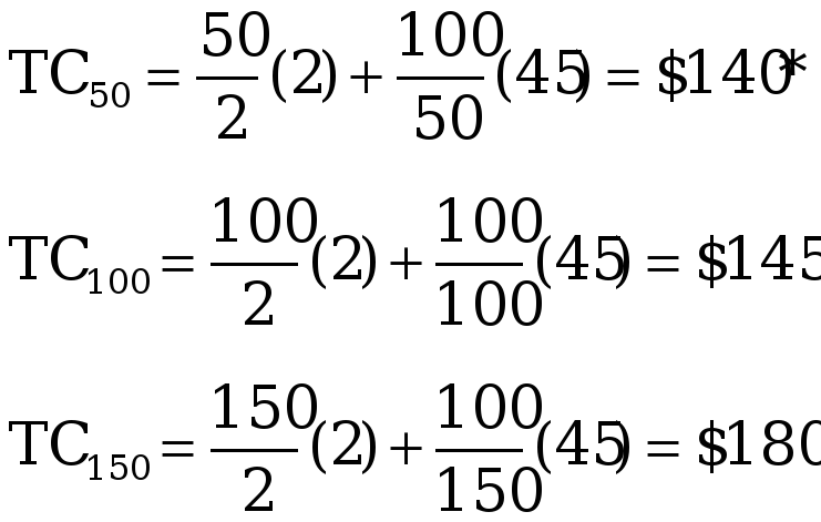
D1 = 100/month (months 1–6)
D2 = 150/month (months 7–12)
a. ![]()
![]()
b. The EOQ model requires this.
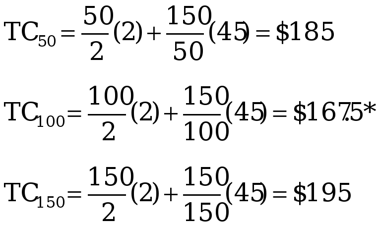
c. Discount of $10/order is equivalent to S – 10 = $45 (revised ordering cost)
1–6 TC74 = $148.32

7–12 TC91 = $181.66

8. D = 27,000 jars/month
H = $.18/month
S = $60
a. ![]()
TC=
TC4,000 = $765.00
Difference
TC4,243 = TC4000 = ![]()
TC4243 = ![]()
b. Current:
Forto equal 10, Q must be 2,700
![]()
Solving, S = $24.30
c. the carrying cost happened to increase rather dramatically from $.18 to approximately $.3705.
![]()
Solving, H = $.3705
9. p = 5,000 hotdogs/day
D= 250/day x 300 days/yr. = 75,000 hotdogs/yr.
u = 250 hotdogs/day300 days per year
S = $66
H = $.45/hotdog per yr.
a. ![]()
b. D/Qo = 75,000/4,812 = 15.59, or about 16 runs/yr.
c. run length: Qo/p = 4,812/5,000 = .96 days, or approximately 1 day
10. p = 50/ton/day
D= 20 tons/day x 200 days/yr. = 4,000 tons/yr.
u = 20 tons/day200 days/yr.
S = $100
H = $5/ton per yr.
a. ![]()
b. ![]()
Average is tons [approx. 3,098 bags]
c. Run length =
d. Runs per year: ![]()
e. Q = 258.2
TC =
TCorig. = $1,549.00
TCrev. = $ 774.50
Savings would be $774.50
11. S = $300
D = 20,000 (250 x 80 = 20,000)
H = $10.00
p = 200/day
u = 80/day
a. ![]()
Q0 = (1,095.451) (1.2910) = 1,414 units
b. Run length =
c. 200 – 80 = 120 units per day
d. ![]()
848 ÷ 80/day = 10.6 days
- 1.0 setup
9.6 days
No, because present demand could not be met.
e. 1) Try to shorten setup time by .40 days.
2) Increase the run quantity of the new product to allow a longer time between runs.
3) Reduce the run size of the other job.]
f. In order to be able to accommodate a job of 10 days, plus one day for setup, there would need to be an11 day supply at Imax, which would be 880 units on hand. Solving the following for Q, we find:
![]()
Q = 1,467.
Using formula 13-4 for total cost, we have
TC @ 1,467 units = $8,489.98
TC @ 1,414 units = $8,483.28
Additional cost = $6.70
12. p = 800 units per day
d = 300 units per day
Q0 = 2000 units per day
a. Number of batches of heating elements per year =batches per year
b. The number of units produced in two days = (2 days)(800 units/day) = 1600 units
The number of units used in two days = (2 days) (300 units per day) = 600 units
Current inventory of the heating unit = 0
Inventory build up after the first two days of production = 1,600 – 600 = 1,000 units
Total inventory after the first two days of production = 0 + 1,000 = 1,000 units.
c. Maximum inventory or Imax can be found using the following equation:

d. Production time per batch =
Setup time per batch = ½ day
Total time per batch = 2.5 + 0.5 = 3 days
Since the time of production for the second component is 4 days, total time required for both components is 7 days (3 + 4). Since we have to make 37.5 batches of the heating element per year, we need (37.5 batches) x (7 days) = 262.5 days per year.
262.5 days exceed the number of working days of 250, therefore we can conclude that there is not sufficient time to do the new component (job) between production of batches of heating elements.
An alternative approach for part d is:
The max inventory of 1,250 will last 1250/300 = 4.17 days
4.17 – .50 day for setup = 3.67 days. Since 3.67 is less than 4 days, there is not enough time.
D = 18,000 boxes/yr.
S = $96
H = $.60/box per yr.
Qo =
![operations management 31]()
Since this quantity is feasible in the range 2000 to 4,999, its total cost and the total cost of all lower price breaks (i.e., 5,000 and 10,000) must be compared to see which is lowest.
TC2,400 = ![]()
TC5,000 = ![]()
TC10,000 = ![]()
H
Lowest TC
ence, the best order quantity would be 5,000 boxes. b. ![]()
| 14. | a. | S = $48 | ||||||||||||
| | | |||||||||||||
| | | D = 25 stones/day x 200 days/yr. = 5,000 stones/yr. | ||||||||||||
| | | | | | | | | |||||||
| | | Quantity | | Unit Price | | a. | H = $2 | |||||||
| | | 1 – 399 | | $10 | | | | |||||||
| | | 400 – 599 | | 9 | | | | |||||||
| | | 600 + | | 8 | | | ||||||||
| | | |||||||||||||
| | TC490 = | 490 | 2 + | 5,000 | 48 + 9 (5,000) = $45,980 | |||||||||
| | 2 | 490 | ||||||||||||
| | | |||||||||||||
| | TC600 = | 600 | 2 + | 5,000 | 48 + 8 (5,000) = $41,000 | |||||||||
| | 2 | 600 | ||||||||||||
| | 600 is optimum. | |||||||||||||
| | | |||||||||||||
| | b. | H | ||||||||||||

| | | (Feasible) | ||||||||||
| | | Compare total costs of the EOQ at $9 and lower curve’s price break: | ||||||||||
| | TC = | Q | (.30P) + | D | (S) +PD | |||||||
| | 2 | Q | ||||||||||
| | | |||||||||||
| | TC422 = | 422 | [.30($9)] + | 5,000 | ($48) + $9(5,000) = $46,139 | |||||||
| | 2 | 422 | ||||||||||
| | | |||||||||||
| | TC600 = | 600 | [.30($8)] + | 5,000 | ($48) + $8(5,000) = $41,120 | |||||||
| | 2 | 600 | ||||||||||
| | Since an order quantity of 600 would have a lower cost than 422, 600 stones is the optimum order size. | |||||||||||
| | c. | ROP = 25 stones/day (6 days) = 150 stones. | ||||||||||
| | | | | | | | | | |
| 15. | | | Range | | P | | H | | Q |
| | | D = 4,900 seats/yr. | 0–999 | | $5.00 | | $2.00 | | 495 |
| | | H = .4P | 1,000–3,999 | | 4.95 | | 1.98 | | 497 NF |
| | | S = $50 | 4,000–5,999 | | 4.90 | | 1.96 | | 500 NF |
| | | | 6,000+ | | 4.85 | | 1.94 | | 503 NF |
| | | Compare TC495 with TC for all lower price breaks: | ||||||||
| | TC495 = | 495 | ($2) + | 4,900 | ($50) + $5.00(4,900) = $25,490 | |||||
| | 2 | 495 | ||||||||
| | TC1,000 = | 1,000 | ($1.98) + | 4,900 | ($50) + $4.95(4,900) = $25,490 | |||||
| | 2 | 1,000 | ||||||||
| | TC4,000 = | 4,000 | ($1.96) + | 4,900 | ($50) + $4.90(4,900) = $27,991 | |||||
| | 2 | 4,000 | ||||||||
| | TC6,000 = | 6,000 | ($1.94) + | 4,900 | ($50) + $4.85(4,900) = $29,626 | |||||
| | 2 | 6,000 | ||||||||
Hence, one would be indifferent between 495 or 1,000 units
16. D = (800) x (12) = 9600 units
S = $40
H = (25%) x P
For Supplier A:

For Supplier B:

Since $132,178 < $133,141.85, choose supplier A.
The optimal order quantity is 500 units.
17. D = 3600 boxes per year
Q = 800 boxes (recommended)
S = $80 /order
H = $10 /order
If the firm decides to order 800, the total cost is computed as follows:

Even though the inventory total cost curve is fairly flat around its minimum, when there are quantity discounts, there are multiple U shaped total inventory cost curves for each unit price depending on the unit price. Therefore when the quantity changes from 800 to 801, we shift to a different total cost curve.
If we take advantage of the quantity discount and order 801 units, the total cost is computed as follows:

The order quantity of 801 is preferred to order quantity of 800 because TCQ=801 < TCQ=800 or 7964.55 < 8320.

The order quantity of 800 is not around the flat portion of the curve because the optimal order quantity (EOQ) is much lower than the suggested order quantity of 800. Since the EOQ of 240 boxes provides the lowest total cost, it is the recommended order size.
18. Daily usage = 800 ft./day Lead time = 6 days
Service level desired: 95 percent. Hence, risk should be 1.00 – .95 = .05
This requires a safety stock of 1,800 feet.
ROP = expected usage + safety stock
= 800 ft./day x 6 days + 1,800 ft. = 6,600 ft.
19. Expected demand during LT = 300 units
dLT = 30 units
a. Z = 2.33, ROP = exp. demand + Z d LT
300 + 2.33 (30) = 369.9 = 370 units
b. 70 units (from a.)
c. smaller Z = less safety stock
ROP smaller:
20. LT demand = 600 lb.
d LT = 52 lb.
risk = 4% Z = 1.75
a. ss = Z d LT = 1.75 (52 lbs.) = 91 lbs.
b. ROP = Average demand during lead time + safety stock
ROP = 600 + 91 = 691 lbs.
With no safety stock risk is 50%.
21. ( = 21 gal./wk.
d = 3.5 gal./wk.
LT = 2 days
SL = 90 percent requires z = +1.28
a. ![]()
b. ![]()
or approx. 34 gal./wk.
Average demand per day = 21 gallons / 7days per week = 3 gallons
= Average demand during lead time = (3 gallons) (2 days) = 6 gallons

Z is approximately 1.07. From Appendix B, Table B, the lead time service level is .8577. Risk of stockout is 1 - .8577 = .1423
c. 1 day after From a, ROP = 8.39
2 more days
on hand = ROP – 2 gal. = 6.39 6.39 = 21 (2/7) + Z (3.5)
P (stockout) = ? ![]()
d = 21 gal./wk. From Appendix B, Table B, Z=.21 gives a risk of
d= 3.5 gal./wk. 1 – .5832 = .4168 or about 42%
| 22. | d = 30 gal./day | ||
| | ROP = 170 gal. | ||
| | LT = 4 days | ss = Z d LT = 50 | |
| | ss = 50 gal. | ||
| | Risk = 9% Z = 1.34 | Solving, d LT = 37.31 | |
| | 3% Z = 1.88 x 37.31 = 70.14 gal. | ||
| | | ||
23. D = 85 boards/day ROP = d x + Z d LT
ROP = 625 boards 625 = 85 x 6 + Z (85) 1.1
= 6 days Z = 1.23 10.93%
LT= 1.1 day .1093 approx. 11%
24. SL 96% Z = 1.75 ROP = + Z
= 12 units/day
= 4 days = 12 (4) + 1.75
d= 2 units/day LT = 1 day = 48 + 1.75 (12.65)
= 48 + 22.14
= 70.14
25. LT = 3 days S = $30
D = 4,500 gal H = $3
360 days/yr.
d= 2 gal.
Risk = 1.5% Z = 2.17
a. Qty. Unit Price Qo =
1 – 399 $2.00
400 – 799 1.70
800+ 1.62
TC = Q/2 H + D/Q S + PD
TC300 = 150 (3) + 15 (30) + 2(4,500) = $9,900
TC400 = 200(3) + 11.25(30) + 1.70(4,500) = $8,587.50*
TC800 = 400(3) + 5.625(30) + 1.62(4,500) = $8,658.75
b. ROP = LT + Z
= 12.5 (3) + 2.17 (2)
= 37.5 + 7.517
= 45.02 gal.
26. d = 5 boxes/wk.
d= .5 boxes/wk.
LT = 2 wk.
S = $2
H = $.20/box
a. D = .5 boxes/wk. x 52 wk./yr. = 26 boxes/yr.
![]()
| | b. | ROP = |
![]()
| | | ||
| | | Area under curve to left is .9977, so risk = 1.0000 – .9977 = .0023 | |
c. ![]()
| | | Thus, |
36 = 5(7 + 2) + z(.5) – 12
| | | ||
| | | Solving for z yields z = +2.00 which implies a risk of 1.000 – .9772 = .0228. | |
| 27. | | ||||||||||||
| | d= 10 lb. | ||||||||||||
| | | ||||||||||||
| | LT = 1 day | ||||||||||||
| | SL = 90 percent, so z = +1.28 | ||||||||||||
| | | ||||||||||||
| | a. | ROP = | |||||||||||
| | | | = 80 (8) + 1.28 | ||||||||||
| | | | = 748.61 [round to 749] | ||||||||||
| | b. | E(n) = E(z) dLT = .048(84.85) = 4.073 units | |||||||||||
| | | | |||||||||||
| 28. | D = 10 rolls/day x 360 days/yr. = 3,600 rolls/yr. | ||||||||||||
| | | LT = 3 days | H = $.40/roll per yr. | ||||||||||
| | d = 2 rolls/day | S = $1 | |||||||||||
| | a. |
| |||||||||||
| | | ||||||||||||
| | b. | SL of 96 percent requires z = +1.75 | |||||||||||
| | | ROP = | |||||||||||
| | c. | E(n) = E(z) d LT = .016( | |||||||||||
| | | E(N) = E(n) | D | = .0554 | 3600 | = 1.488 or about 1.5 rolls | |||||||
| | | Q | 134 | ||||||||||
| | d. | | | ||||||||||
| | |||||||||||||
| 29. | (Partial Solution) | Qo= 179 cases | |||||||||||
| | SLannual = 99% | SLannual = 1 – | E(z) d LT | ||||||||||
| | | Q | |||||||||||
| | a. | SS = ? | b. | risk = ? | .99 = 1 – | E(z) d LT | |||||||
| | | | 179 | ||||||||||
| | dLT = 80, d LT = 5 | Solving, E(z) = 0.358 | |||||||||||
| | | From Table 12–3, Z = 0.08 Hence, the probability of a stockout is 1-.8577=.1423. | |||||||||||
| | | | |||||||||||
| | a. | ss = Z d LT | | ||||||||||
| | | = .08 (5) = .40 cases | |||||||||||
| | b. | 1 – .5319 = .4681 | |||||||||||
| 30. | | H = $1/month | D = 250 gal./wk. x 52 wk./yr. = 13,000 gal./yr. | ||||||||||||||||
| | d= 14 gal./wk. | S = $20 | | ||||||||||||||||
| | LT = 10 wk. .5 Yes | | |||||||||||||||||
| | SLannual = 98% | ||||||||||||||||||
| | | ||||||||||||||||||
| | a. | SLannual = 1 – | (z) dLT | ||||||||||||||||
| | Q | ||||||||||||||||||
| | | | | .02 = | (z) 9.90 | ||||||||||||||
| | | = | | 208 | |||||||||||||||
| | | = 9.90 | | E(z) = .42 z = –.04 | SS = –.04(9.90) = –.40 | ||||||||||||||
| | | | SL = .4840 | | |||||||||||||||
| | b. | E(n) = E(z) dLT | |||||||||||||||||
| | | 5 = E(z)9.90 | |||||||||||||||||
| | | E(z) = .505 z = –.20 | SS = zdLT | ||||||||||||||||
| | | SL = .4207 | SS = –.20(9.90) = –1.98 units | ||||||||||||||||
| 31. | FOI | | Q = | ||||||||||||||||
| | SL = .98 | | = Cycle | ||||||||||||||||
| | OI = 14 days | | 1 | 640 + 2.05(3) | |||||||||||||||
| | LT = 2 days | | 2 | 640 + 2.05(3) | |||||||||||||||
| | D = 40/day | | 3 | 640 + 2.05(3) | |||||||||||||||
| | d = 40/day | | | ||||||||||||||||
2= 3/day
| 32. | 50 wk./yr. | | |||||||||
| | P34 | | P35 | | | ||||||
| | D = 3,000 units | | D = 3,500 units | | | ||||||
| | | | | | | ||||||
| | d = 4 units/wk. | | d = 5 units/wk. | | | ||||||
| | LT = 2 wk. | | LT = 2 wk. | | | ||||||
| | unit | | unit | | | ||||||
| | cost = $15 | | cost = $20 | | | ||||||
| | H = (.30)(15) = $4.50 | | H = (.30)(20) = 6.00 | | | ||||||
| | S = $70 | | S = $30 | | | ||||||
| | Risk = 2.5% | | Risk = 2.5% | | | ||||||
| | | | | Q = (OI + LT) | |||||||
| | | | |||||||||
| | QP35 = 70 (4 + 2) + 1.96 | ||||||||||
| | ROPP34 = | | | QP35 = 420 + 24 – 110 | |||||||
| | | | | QP35 = 334 units | |||||||
| | ROPP34 = 60(2) + 1.96 | | | ||||||||
| 33. a. | Item | Annual $ volume | Classification | | |
| | H4-010 | 50,000 | C | | |
| | H5–201 | 240,800 | B | | |
| | P6-400 | 279,300 | B | | |
| | P6-401 | 174,000 | B | | |
| | P7-100 | 56,250 | C | | |
| | P9-103 | 165,000 | C | | |
| | TS-300 | 945,000 | A | | |
| | TS-400 | 1,800,000 | A | | |
| | TS-041 | 16,000 | C | | |
| | V1-001 | 132,400 | C | | |
| | | | | | |
| b. | Item | Estimated annual demand | Ordering cost | Unit holding cost ($) | EOQ |
| | H4-010 | 20,000 | 50 | .50 | 2,000 |
| | H5-201 | 60,200 | 60 | .80 | 3,005 |
| | P6-400 | 9,800 | 80 | 8.55 | 428 |
| | P6-401 | 14,500 | 50 | 3.60 | 635 |
| | P7-100 | 6,250 | 50 | 2.70 | 481 |
| | P9-103 | 7,500 | 50 | 8.80 | 292 |
| | TS-300 | 21,000 | 40 | 11.25 | 386 |
| | TS-400 | 45,000 | 40 | 10.00 | 600 |
| | TS-041 | 800 | 40 | 5.00 | 113 |
| | V1-001 | 33,100 | 25 | 1.40 | 1,087 |
| | | | | | |
| 34. | | | | | |
| Cs = Rev – Cost = $4.80 – $3.20 = $1.60 | ||||||||||||||
| Ce = Cost – Salvage = $3.20 – $2.40 = $.80 | ||||||||||||||
| | SL = | Cs | = | $1.60 | = | 1.6 | = .67 | | x | | | | Cum. | |
| | Cs + Ce | $1.60 + $.80 | 2.4 | | Demand | | P(x) | | P(x) | |||||
| | | | | | | | 19 | | .01 | | .01 | |||
| | Since this falls between the cumulative | | 20 | | .05 | | .06 | |||||||
| | probabilities of .63(x = 24) and .73(x = 25), | | 21 | | .12 | | .18 | |||||||
| | this means Don should stock 25 dozen doughnuts. | | 22 | | .18 | | .36 | |||||||
| | | | 23 | | .13 | | .49 | |||||||
| | | | 24 | | .14 | | .63 | |||||||
| | | | 25 | | .10 | | .73 | |||||||
| | | | 26 | | .11 | | .84 | |||||||
| | | | 27 | | .10 | | .94 | |||||||
| | | | . | | . | | . | |||||||
| | | | . | | . | | . | |||||||
| | | | . | | . | | . | |||||||
| 35. | Cs = $88,000 | | ||||||||
| | Ce = $100 + 1.45($100) = $245 | | ||||||||
| a. | SL = | Cs | = | $88,000 | = .9972 | | ||||
| Cs + Ce | $88,000 + $245 | [From Poisson Table with = 3.2] | ||||||||
| | | | x | Cum. Prob. | ||||||
| | Using the Poisson probabilities, the minimum level | | 0 | .041 | ||||||
| | stocking level that will provide the desired service | | 1 | .171 | ||||||
| | is nine spares (cumulative probability = .998). | | 2 | .380 | ||||||
| | | | 3 | .603 | ||||||
| | | | 4 | .781 | ||||||
| | | | 5 | .895 | ||||||
| | | | 6 | .955 | ||||||
| | | | 7 | .983 | ||||||
| | | | 8 | .994 | ||||||
| | | | 9 | .998 | ||||||
| | | | . | . | ||||||
| | | | . | . | ||||||
| | | | . | . | ||||||
b.
Carrying no spare parts is the best strategy if the shortage cost is less than or equal to $10.47 ().
| 36. | Cs = Rev – Cost = $5.70 – $4.20 = $1.50/unit | | | | ||||||||||||||
| | Ce = Cost – Salvage = $4.20 – $2.40 = $1.80/unit | | | d= 10 lb./day | ||||||||||||||
| | SL = | Cs | = | $1.50 | = | $1.50 | = .4545 | |||||||||||
| | Cs + Ce | $1.50 + $1.80 | $3.30 | |||||||||||||||
| | The corresponding z = –.11 | |||||||||||||||||
| | So = | |||||||||||||||||
| | | | ||||||||||||||||
| 37. | | A stocking level of 49 quarts translates into a z of + 1.5: | ||||||||||||||||
| | d = 6 qt./day | | ||||||||||||||||
| | Ce = $.35/qt | z = | S – | = | 49 – 40 | = 1.5 | ||||||||||||
| | Cs = ? | d | 6 | |||||||||||||||
| | S = 49 qt. | This implies a service level of .9332: | ||||||||||||||||
| | SL = | Cs | Thus, .9332 = | Cs | |
| | Cs + Ce | Cs+ $.35 | |||
| | Solving for Cs we find: .9332(Cs + .35) = Cs; Cs = $4.89/qt. | ||||
| | | ||||
| | Customers may buy other items along with the strawberries (ice cream, whipped cream, etc.) that they wouldn’t buy without the berries. | ||||
| 38. | Cs = Rev – Cost = $12 – $9 = $3.00/cake | ||||||||||||||||||||
| | Ce = Cost – Salvage = $9 – ½ ($9.00) = $4.50/cake | ||||||||||||||||||||
| | Demand is Poisson with mean of 6 | [From Poisson Table with = 6.0] | |||||||||||||||||||
| | SL = | Cs | = | $3.00 | = .40 | | Demand | Cum. Prob. | | ||||||||||||
| | Cs + Ce | $3.00 + $4.50 | | 0 | .003 | | |||||||||||||||
| | | | | | | | 1 | .017 | | ||||||||||||
| | Since .40 falls between the cumulative probability for demand of 4 and 5, the optimum stocking level is 5 cakes. | | 2 | .062 | | ||||||||||||||||
| | | 3 | .151 | | |||||||||||||||||
| | | 4 | . | .40 | |||||||||||||||||
| | | | | | | | 5 | .446 | |||||||||||||
| | | | | | | | 6 | .606 | | ||||||||||||
| | | | | | | | . | . | | ||||||||||||
| | | | | | | | . | . | | ||||||||||||
| | | | | | | | . | . | | ||||||||||||
| | Cs = $.10/burger x 4 burgers/lb. = $.40/lb. | ||||||||||||||||||||
| | Ce = Cost – Salvage = $1.00 – $.80 = $.20/lb. | ||||||||||||||||||||
| | SL = | Cs | = | $.40 | = .6667. | ||||||||||||||||
| | Cs + Ce | $.40 + $.20 | |||||||||||||||||||
| | The appropriate z is +.43. | ||||||||||||||||||||
| | So = + z = 400 + .43(50) = 421.5 lb. | ||||||||||||||||||||
| 40. | Cs = $10/machine | Demand | Freq. | Cum. Freq. | |||||||||||||||||
| | Ce = ? | 0 | .30 | .30 | |||||||||||||||||
| | S = 4 machines | 1 | .20 | .50 | |||||||||||||||||
| | | 2 | .20 | .70 | |||||||||||||||||
| | | 3 | .15 | .85 | |||||||||||||||||
| | | 4 | .10 | .95 | |||||||||||||||||
| | | 5 | .05 | 1.00 | |||||||||||||||||
| | | | 1.00 | | |||||||||||||||||
| | a. | For four machines to be optimal, the SL ratio must be .85 | $10 | .95. | |||||||||||||||||
| | $10 + Ce | ||||||||||||||||||||
| | | Setting the ratio equal to .85 and solving for Ce yields $1.76, which is the upper end of the range. | |||||||||||||||||||
| | | Setting the ratio equal to .95 and again solving for Ce , we find Ce = $.53, which is the lower end of the range. | |||||||||||||||||||
| | b. | The number of machines should be decreased: the higher excess costs are, the lower SL becomes, and hence, the lower the optimum stocking level. | |||||||||||||||||||
| | c. | For four machines to be optimal, the SL ratio must be between .85 and .95, as in part a. Setting the ratio equal to .85 yields the lower limit: | |||||||||||||||||||
| | | .85 = | Cs | Solving for Cs we find Cs = $56.67. | |||||||||||||||||
| | Cs + $10 | ||||||||||||||||||||
| | | Setting the ratio equal to .95 yields the upper end of the range: | |||||||||||||||||||
| | | .95 = | Cs | Solving for Cs we find Cs = $190.00 | |||||||||||||||||
| | Cs + $10 | ||||||||||||||||||||
41. a. Ratio Method
# of spares Probability of Demand Cumulative Probability
0 0.10 0.10
1 0.50 0.60
2 0.25 0.85
3 0.15 1.00
Cs = Cost of stockout = ($500 per day) (2 days) = $1000
Ce = Cost of excess inventory = Unit cost – Salvage Value = $200 – $50 = $150
![]()
Since 86.9% is between cumulative probabilities of 85% and 100%, we need to order 3 spares.
Tabular Method
| Stocking | Demand = 0 | Demand = 1 | Demand = 2 | Demand = 3 | Expected |
| Level | Prob. = 0.10 | Prob. = 0.50 | Prob. = 0.25 | Prob. = 0.15 | Cost |
| 0 | $0 | .50(1)($1000)=$500 | .25(2)($1000)=$500 | .15(3)($1000)=$450 | $1,450 |
| 1 | .10(1)($150)=$15 | $0 | .25(1)($1000)=$250 | .15(2)($1000)=$300 | $565 |
| 2 | .10(2)($150)=$30 | .50(1)($150)=$75 | $0 | .15(1)($1000)=$150 | $255 |
| 3 | .10(3)($150)=$45 | .50(2)($150)=$150 | .25(1)($150)=$37.50 | $0 | $232.50 |
We should order 3 spares.
a. Ratio Method: Demand and the probabilities for the cases of wedding cakes are given in the following table.
Demand Probability of Demand Cumulative Probability
0 0.15 0.15
1 0.35 0.50
2 0.30 0.80
3 0.20 1.00
Cs = Cost of stockout = Selling Price – Unit Cost = $60 – $33 = $27
Ce = Cost of excess inventory = Unit Cost – Salvage Value = $33 – $10 = $23
![]()
Since the service level of 54% falls between cumulative probabilities of 50% and 80%, the supermarket should stock 2 cases of wedding cakes.
Tabular Method
| Stocking | Demand = 0 | Demand = 1 | Demand = 2 | Demand = 3 | Expected |
| Level | Prob. = 0.15 | Prob. = 0.35 | Prob. = 0.30 | Prob. = 0.20 | Cost |
| 0 | $0 | .35(1)($27)=$9.45 | .30(2)($27)=$16.20 | .20(3)($27)=$16.20 | $41.85 |
| 1 | .15(1)($23)=$3.45 | $0 | .30(1)($27)=$8.10 | .20(2)($27)=$10.80 | $22.35 |
| 2 | .15(2)($23)=$6.90 | .35(1)($23)=$8.05 | $0 | .20(1)($27)=$5.40 | $20.35 |
| 3 | .15(3)($23)=$10.35 | .35(2)($23)=$16.10 | .30(1)($23)=$6.90 | $0 | $33.35 |
The supermarket should stock 2 cases of wedding cakes.
43. Cs = $99, Ce = $200
| SL = | 99___ 99 + 200 | = 0.3311. z = −0.44. |
| Overbook: 18 – 0.44(4.55) = 15.998, or 16 tickets. |
44. Mean usage = 4.6 units/day
Standard dev. = 1.265 units/day
LT = 3 days
ROP = 18
Using equation 12-13: 18 = 4.6(3) + z(1.265)√3
Solving, z = 1.92 which gives a service level of 97.26%.
1 Students must recognize that without demand variability, the fixed order interval order quantity equation reduces to:
Q = d(LT + OI) – Available (because there is no safety stock)
Since Available = d x LT, the fixed order interval order quantity equation Q further reduces to the following:
Q = d x OI = (6) (89) = 534 units
Therefore, ordering at six-week intervals requires an order quantity of 534 units.
On the other hand, the optimal order quantity is determined by using the basic EOQ equation.
![]()
The weekly total cost based on optimal order quantity EOQ is given below:

The weekly total cost based on six-week fixed order interval (FOI) order quantity is given below:

Weekly savings of using EOQ rather than 6-week FOI is 26.69 – 21.35 = $5.34
The annual savings = (52 weeks) ($5.34 /week) = $277.68
2. The total annual savings as a result of switching from six-week FOI to EOQ are relatively small and switching to the optimal order quantity may not be warranted. However, even though the absolute value of the savings is relatively small, the percentage of savings is approximately 25% (5.34 / 21.35). Therefore if FOI approach is used with other parts or components as well, the total potential loss may be significant.
In order to improve the current inventory control system, the new president may want to consider the following:
1. Computerize the inventory control system. There are too many parts for the current manual system.
2. Currently, no paper work is used when items are withdrawn from the stockroom when they are needed on the shop floor. Harvey Industries may either want to establish a procedure for recording the transactions in the stockroom or invest in a bar coding system. If a bar coding system is purchased, it has to be coordinated with the new computerized inventory control system. Establishing a cycle counting procedure may be very helpful also. As a result of these actions, the inventory accuracy should substantially improve.
3. It appears that utilization of ABC inventory classification system is needed. The company should never experience stockouts in their basic “C” items. ABC analysis will allow Harvey Industries to establish an appropriate degree of control over items in terms of order quantity and ordering frequency.
Case: Grill RiteThe president’s stance on steady output conflicts with seasonal demand. However, it is unlikely that this will change. One alternative might be to identify a complementary product that would offset seasonal demand for electric grills.
The main problem is inventory management. One advantage of having a single, centralized warehouse is the lower need for safety stock due to the canceling effect of random variability in orders from the various regions. Conversely, with separate warehouses, each warehouse needs a relatively larger safety stock to guard against variations in demand. What is needed is overall control of the system that would take into account seasonal variations in demand and achieve a better match between regional demand and supply. This might involve making or improving regional forecasts. In any case, improved system visibility is essential: direct access to regional warehouse data by the main warehouse is needed in order to be able to coordinate and set priorities on inventory shipments to regional warehouses. That should take care of most of the problem. It may also pay to examine the feasibility of shipping from one warehouse to another when a shortage occurs. Relevant costs would include transaction costs, transportation costs, versus the potential increase in profit by making up a shortage.
Case: Farmers Restaurant
1. Inventories are crucial not only to Farmers Restaurant, but to businesses in general. Customer satisfaction and customer return is contingent upon proper inventory management. If customers visit the Farmers Restaurant and are unable to receive the food they desire due to stockout, the customer may be dissatisfied and may not return to Farmers Restaurant. In addition to customer satisfaction, total food costs are also important to businesses. In the restaurant industry if too much of a product is ordered and not used; it could result in product wastage due to the items expiring. This would result in an increase in total food costs when the goal is to keep food costs low! Overstocking products can also negatively affect Farmers Restaurant and other businesses. By having more products on-hand than needed, Farmers Restaurant is tying up funds that might be more productive elsewhere. Overall, it is imperative that Farmers Restaurant try to successfully manage inventory levels due to these potential/existing problems.
2. A fixed-interval ordering system is appropriate.
3. Q = ˉd (OI + LT) + zσd √(OI + LT) – A
OI = Time between orders
LT = Lead Time
It is expected demand between orders and lead time + safety stock – inventory on hand
Q = 5 (3+2) + 1.64 (3.5) √(3 + 2) – 3
= 25 + 13 – 3
= 35 (Therefore, 18 2-packs.)
4. 12 = 5 x 2 + z (3.5) (1.41)
12 = 10 + z (4.935)
2 / 4.935 = z (4.935) / 4.935
Z = 0.41
Service Level = 0.6554
1 – 0.6554 = 0.3446
Therefore, the risk for stockout is 34.46% which is high
Operations Tour: Bruegger’s Bagel Bakery1. If too little inventory is maintained, there is a risk of stockout and potential lost sales. In addition, if there is not sufficient work-in-process inventory, the production process may become too inefficient, raising the cost of production. On the other hand, if too much inventory is maintained, the carrying cost may become excessively high.
2. a. Customers judge the quality of bagels by their appearance (size, shape and shine), taste and consistency. Customers are also very interested in receiving high service quality.
b. At each stage of the production process, workers check bagel quantity.
c. Steps for Bruegger’s Bagel Bakery Operations:
Purchase ingredients from suppliers
Mix the dough
Shape the dough
Ship to stores
Store the bagels
Boil and malt
Bake
Sell to customers
The company can improve quality at each step by monitoring output more carefully and training and education of the employees.
3. The basic ingredients can be purchased using either fixed order interval or fixed order quantity models. EOQ production lot size model is most appropriate for deciding the size of production quantity.
4. If there is a bagel-making machine at each store, the company would have to invest in more machinery, more space for production and storage, and more worker training for the production of bagels. However, the lead time to make the bagels will be shortened. The shorter lead time will provide faster, more flexible response to customer demands and fresher bagels.
Enrichment Module: Advanced EOQ ProblemThis enrichment module consists of an additional EOQ problem to further solidify the concepts associated with the Economic Production Model. The question forces the students to work backwards through the EOQ production equation.
A company produces plastic powder in lots of 2000 pounds, at the rate of 250 pounds per hour. The company uses powder in an injection molding process at the steady rate of 50 pounds per hour for an eight-hour day, five days a week. The manager has indicated that the setup cost is $100 for this product, but “We really have not determined what the holding cost is.”
a. What weekly holding cost per pound does the lot size imply, assuming the lot size is optimal?
b. Suppose the figure you compute for holding cost has been shown to the manager, and the manager says that it is not that high. Would that mean the lot size is too large or too small? Explain.
Solution to Enrichment Module Problema.

b. Decreasing the value of carrying cost (H) will result in an increase in the lot size. Since holding inventory is not as expensive, the firm can afford to carry more inventory and therefore produce a larger batch.
In most cases, shortages are undesirable and should be avoided. However, in certain circumstances, it may be desirable to plan and allow for shortages. Planned shortages are implemented for high dollar volume items where the inventory carrying cost is very high. The model discussed in this section refers to the specific type of shortages called backorders. When a customer attempts to purchase an out‑of‑stock item, the firm does not lose the sale. The customer waits until the purchased order arrives from the supplier. If there were no additional cost associated with backordering, there would be no incentive for the firm to maintain any inventory. However, there are costs associated with backordering. The tangible part of the backorder cost involves the cost of expediting the delivery (special delivery) and production of the backordered item. The intangible part of the backordering cost involves the loss of goodwill due to the fact that the customers are forced to wait for their orders. The longer the waiting period, the higher the backorder cost due to loss of goodwill.
There is a direct trade‑off between the inventory carrying cost and the cost of a planned shortage in the form of backorders. In many cases the cost of backorders can be easily offset by the reduction in carrying costs. The model discussed in this section will not be valid if a customer decides not to wait for the backorder.
The fixed order quantity inventory model with planned shortages (backorders) is very similar to the basic EOQ model. When the reorder point is reached, a new economic order quantity (Q) is placed. Figure 1 shows the schematic representation of this model. The size of the backorder is B units and the maximum inventory is Q–B units. The average size of the backorder is B/2 for each order cycle. T is defined as the amount of time between two successive orders (a complete order cycle). t1 is the part of the order cycle where the customer orders are met from stock. In other words, during t1 there is positive inventory level. On the other hand, t2 is the period of time in the order cycle where the inventory is depleted and all the customer orders are placed on backorder (stockout period).
Symbol definitions used to explain various concepts are listed below.
H = carrying cost per unit per year
S = setup cost per batch (lot)
D = annual demand
Q* = optimal order quantity
B = size of the backorder
CB = backorder cost per unit per year
B* = optimal planned backorder quantity
T = Q/D (length of the complete order cycle in years) or
T = Q/d (length of the complete order cycle in days)
t1 = (Q – B)/D or (Q – B)/d (time period during which inventory is positive)
t2 = B/D or B/d (time period during which there is no inventory)
In this model, the average inventory is not Q/2 or not even (Q – B)/2 because during the shortage period there are no units in inventory. The average inventory calculation for this model can be explained with the following example:
A large local car dealership orders a certain brand of automobiles from a car manufacturer located in Detroit. Order quantity (Q) is 500 units, annual demand (D) is 7500 and the firm operates 300 working days per year. Due to the high holding costs, the company plans to backorder (B) 200 cars per order cycle. Determine the average inventory.
d = (D/number of operational days) = 7,500/300 = 25 units (daily consumption)
T = Q/d = 500/25 = 20 days. (time between orders is 20 days)
t1 = (Q – B)/d = (500 – 200)/25 = 300/25 = 12 days (time period during which there is no shortage)
t2 = B/d = 200/25 = 8 days (time period during which there is no inventory)
The dealership will carry an average of (Q – B)/2 units during t1 and no units during t2. Therefore, total number of unit days during the inventory cycle can be computed by multiplying t1 with (Q – B)/2

In other words, an average of 150 units are carried in inventory for 12 days and zero units are carried for 8 days (shortage period). Therefore, total number of unit days of inventory during the complete order cycle is (150)(12) = 1800.
Since there are a total of 20 days in the complete order cycle, the average inventory can be computed by dividing the total number of unit days of inventory by the number of days in the inventory cycle. In this example, the average inventory is equal to 1,800/20 or 90 units. Therefore, the average inventory can be computed by using the following formula:

Using a similar logic, we can also develop the average backlog formula. The dealership will experience shortage (backorders) for 8 days during the order cycle. The average amount of backorder on a given shortage day is B/2. Based on this information, the total number of backorder unit days can be computed using the following equation: (t2) (B/2) = (B/D)(B/2) = B2 /2D.
In our example, there are 8 days of a planned shortage period. During this period, an average of 200/2 = 100 units of backorders are realized. Therefore, the total number of backorder unit days during the order cycle is (8)(100) = 800 units. Since there are a total of 20 days in the order cycle, the average backorder quantity for the complete order cycle can be determined by dividing the total number of backorder unit days by the number of days in the complete inventory cycle. In this example, using the above equation, we obtain an average backorder quantity of 800/20 = 40 units. The general equation for the average backorder quantity is:

Annual inventory carrying cost is still calculated by multiplying the average inventory with the inventory carrying cost per unit per year. The formula for the annual ordering (setup) cost is the same as it was for the basic EOQ model. The annual backorder cost is determined by multiplying the average backorder quantity with the backorder cost per unit per year.
The annual inventory carrying cost is given by:
The annual ordering and backordering costs are given by the following respective formulas:
Therefore, the total annual inventory cost (TC) can be expressed by summing the annual inventory carrying cost, annual ordering cost and the annual backordering cost as shown in the following formula:
![]()
Taking the first total derivative of the above total cost formula with respect to Q and setting the resulting equation to zero and solving for Q will result in the following optimal quantity (Q*) and optimal backorders (planned shortages) (B*) formulas:
Figure 1
An inventory situation with planned shortages
Example:
XYZ Company distributes a major part for the F–15 fighter jets. Due to the very high holding cost, the company wants to implement a model with planned shortages. The annual demand is 78,000 and the company operates 300 days per year. The annual carrying rate is 10% of the item cost and the unit cost of this item is $1,000. The setup cost per batch is estimated at $500.
a. Determine the optimal order quantity and total annual inventory cost (setup cost + carrying cost) using the basic EOQ model with no backorders.
b. If each unit backordered costs the company $200 per unit per year, what would be the optimal order quantity and the optimal size of the planned backorder?
c. Determine the annual carrying cost, the annual setup cost, the annual backordering cost and the annual total inventory cost for the planned shortage model used in part b.
d. Determine the values of t1, t2 and T in days.
e. Should the company adopt the planned backorder model of part b or the basic EOQ model of part a which does not allow backorders?
D = 81,000 units
S = $500
d = 81,000/300 days = 27 units per day.
H = ($1,000) (.10) = $100
CB = $200
a. ![]()
annual setup cost = ![]()
annual carrying cost = ![]()

c.

Let TC = Total annual inventory cost
HC = annual inventory holding cost
SC = annual setup cost
BC = annual backordering cost
TC = HC + SC + BC = 24,495.77 + 36,741.35 + 12,247.55 = 73,485.07
d.

e. The model with planned backorders is preferred because the total annual inventory cost of the basic inventory model is substantially higher than the total annual inventory cost of the planned backorder model.
TCbasic EOQ = 90,000
TCbackorder = 73,485.07
90,000 – 73,485.07 = 16,514.93
The total cost savings equal 18.4%
Problems
The manager of an inventory system believes that inventory models are important decision-making aids. Although the manager often uses an EOQ policy, he has never considered a backorder model because of his assumption that backorders are “bad” and should be avoided. However, with upper management’s continued pressure for cost reduction, you have been asked to analyze the economics of a backordering policy for some products that can possibly be backordered. For a specific product with D = 800 units per year, C0 =$150, H = $10, and Cb = $20, what is the economic difference in the EOQ and the planned shortage or backorder model? If the manager adds constraints that no more than 35% of the units may be backordered and that no customer will have to wait more than 20 days for an order, should the backorder inventory policy be adopted? Assume 250 working days per year.
Solution to Problem
D = 800 units/year
C0 = $150
H = $10/unit/year
Cb = $20/unit/year
Planned shortage model:

EOQ model:
![]()
Total cost planned shortage model:
TC = Total annual inventory cost
HC = Annual inventory holding cost
SC = Annual setup cost
BC = Annual backordering cost
HC = ![]()
SC = ![]()
BC = ![]()
TC = HC + SC + BC = 421.68 + 632.45 + 210.78
TC = $1,264.91
Total cost regular EOQ model:
HC = ![]()
SC = ![]()
TC = HC + SC = 774.60 + 774.60 =$1,549.20
TCDifference = 1,549.20 – 1,264.91 = $284.29
Using the planned shortage model will result in savings of $284.29.
Number of orders = ![]()
Expected annual number of units short = (B)
Expected annual number of units short = (63.24)(4.216) = 266.44
d = units/day
t2 =days
Since 19.763 < 20 and < .35, the backorder inventory policy should be adopted.
13-58
