InstructionsPlease refer to the original Willowbrook School Case Study and previous case study assignments as needed  Read the additional background information below Complete the tasks that fol

SPSS Assignment 6 Instructions

Part 1

Follow the steps below to complete your SPSS homework assignment:

1. From Blackboard, download the SPSS HW #6-1 data file. Graduate student Q is interested in researching if an instructional handwashing video is effective in changing the amount of time that students wash their hands. In her study, Q conducted a pre-test. She had a group of student participants wash their hands at a sink. She used a stop watch to count how many seconds they washed their hands. Then, Q played the instructional handwashing video for them. Then, Q conducted a post-test to see if the video would change the amount of time they washed their hands. She used a stop watch to count how many seconds they washed their hands.

Before we can begin paired sample t-test analysis, there are several assumptions we need to test for:

1. Measurement of variables (2 categorical/dependent [same people for pre/post-test] groups; DV is interval/ratio)

2. No outliers (using the Outlier Labeling Rule)

3. Normal distribution of dependent variable (tested by Shapiro-Wilk, calculation of skewness/kurtosis, inspection)

1. We have met the first assumption because we know that we have 2 categorical groups that are the exact same people for the pre-test and post-test and because we know that the DV is interval/ratio (seconds of handwashing).

1. We will check for outliers (using the Outlier Labeling Rule)

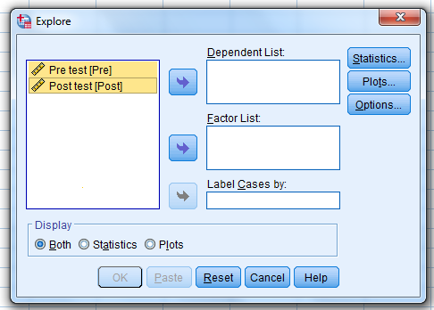
Click on “Analyze,” “Descriptive Statistics,” and “Explore.”

When this pop-up pops up…

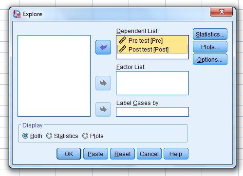
Select the pre-test and post-test…move them…over to the “Dependent List” box

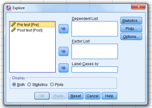
…and then click on “Statistics.”

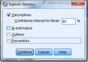
When this pop-up pops up…select “Descriptives”…“Outliers”…“Percentiles”

…and then click “Continue.”

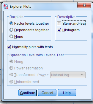
Then, click on “Plots.”

When this pop-up pops up…unselect “Stem-and-leaf”

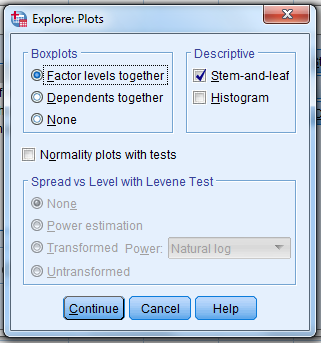
…select “Histogram”…select “Normality plots with tests”

…click “Continue”

…and click “OK.”

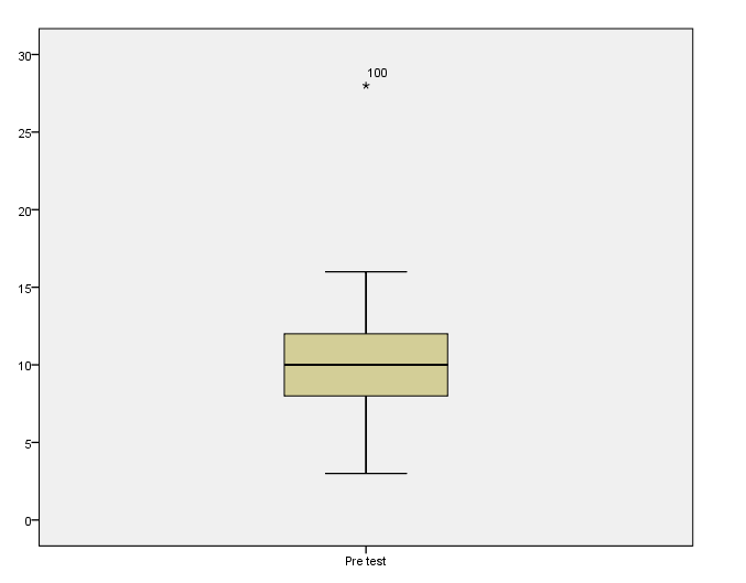
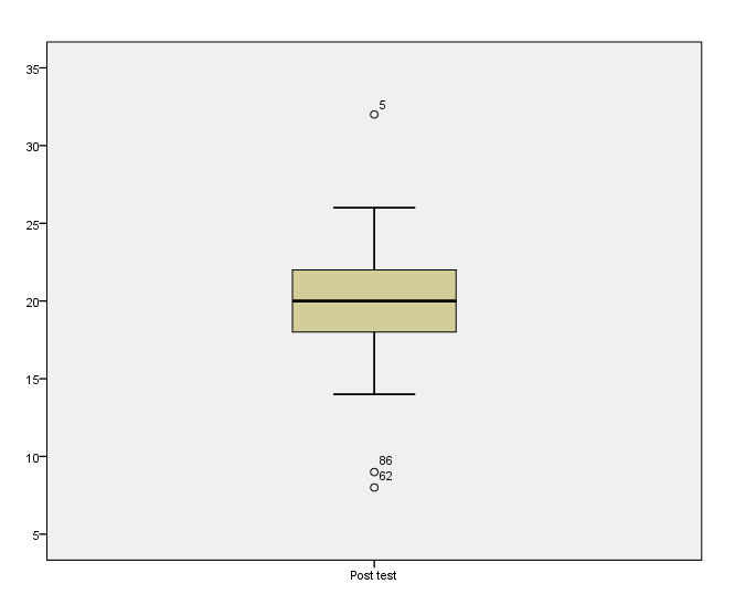
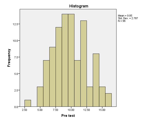
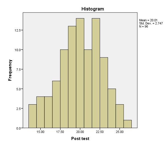
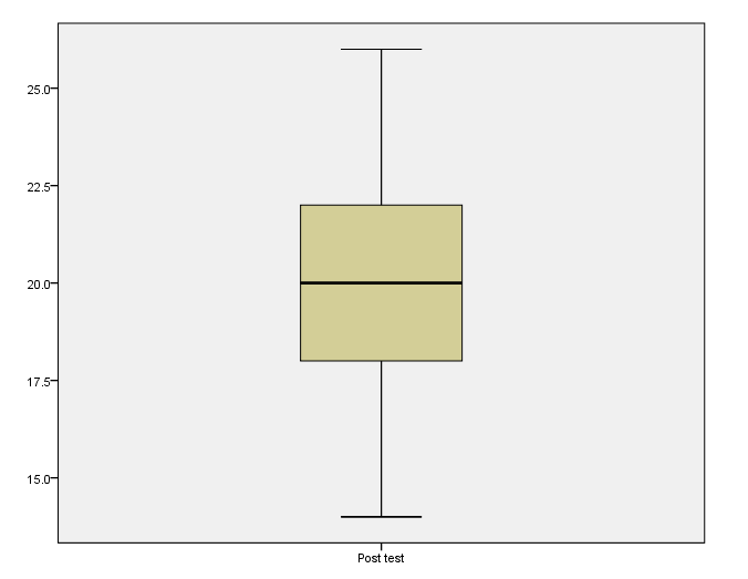
The first indication that you might have outliers will be through inspection of the histogram and box plot.

If you see values on the outskirts of the histograms…

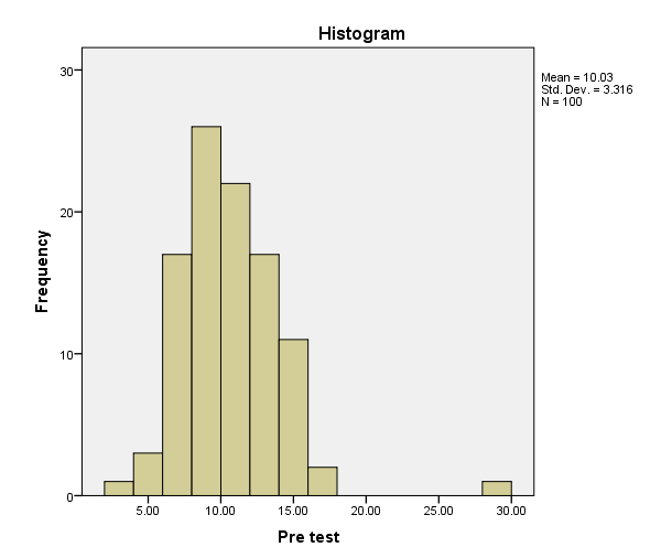
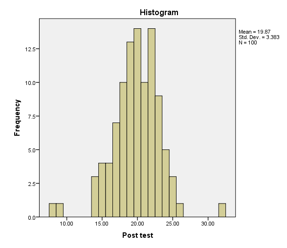
…or dots outside your whiskers, you may have outliers.

To actually test for outliers, we are going to use the Outlier Labeling Rule. We will do this through the “percentiles” table in your SPSS output via a hand calculation to find the upper/lower limits for finding outliers in our data.

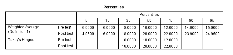
Take the 75th percentile value (Q3) and subtract it from the 25th percentile value (Q1) for the pre-test.

Q3 – Q1 = #

So, in our example:

12 – 8 = 4

Then, take the subtracted value and multiply it by 2.2.

(Q3 – Q1) x 2.2

So, in our example:

(4) x 2.2 = 8.8

Then, take that value and add it to the 75th percentile value (Q3) and subtract it from the 25th percentile value (Q1).

Q3 + ((Q3 – Q1) x 2.2) = upper limit to find outliers

Q1 – ((Q3 – Q1) x 2.2) = lower limit to find outliers

So, in our example:

12 + 8.8 = 20.8

8 – 8.8 = –.8

Repeat this same process for the post-test.

Q3 – Q1 = #

So, in our example:

22 – 18 = 4

Then, take the subtracted value and multiply it by 2.2.

(Q3 – Q1) x 2.2

So, in our example:

(4) x 2.2 = 8.8

Then, take that value and add it to the 75th percentile value (Q3) and subtract it from the 25th percentile value (Q1).

Q3 + ((Q3 – Q1) x 2.2) = upper limit to find outliers

Q1 - ((Q3 – Q1) x 2.2) = lower limit to find outliers

So, in our example:

22 + 8.8 = 30.8

18 – 8.8 = 9.2

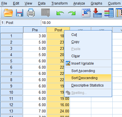
Then, right-click on the pre-test column…click “Sort Descending”

…and delete every case that is above the upper limit that you calculated for the pre-test outliers.

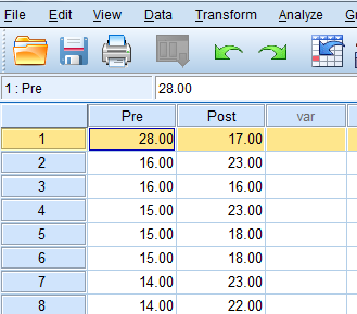
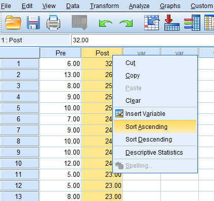
Then, right-click on the pre-test column…click “Sort Ascending”

…and delete the cases that are below the lower limit that you calculated (if there are any).

Now we have to repeat the same steps for removing outliers for the post-test column.

Right-click on the post-test column…click “Sort Descending.”

…and delete every case that is above the upper limit that you calculated for the post-test outliers.

Then, right-click on the post-test column…click “Sort Ascending”

…and delete the cases that are below the lower limit that you calculated.

Now that we have located and deleted outliers, we have met the assumption of no outliers.

1. Now we need to test the assumption of a normal distribution of the dependent variable (tested by Shapiro-Wilk, calculation of skewness/kurtosis, inspection).

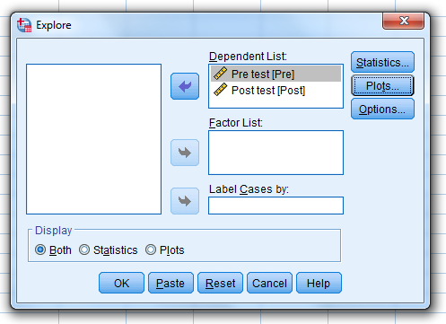
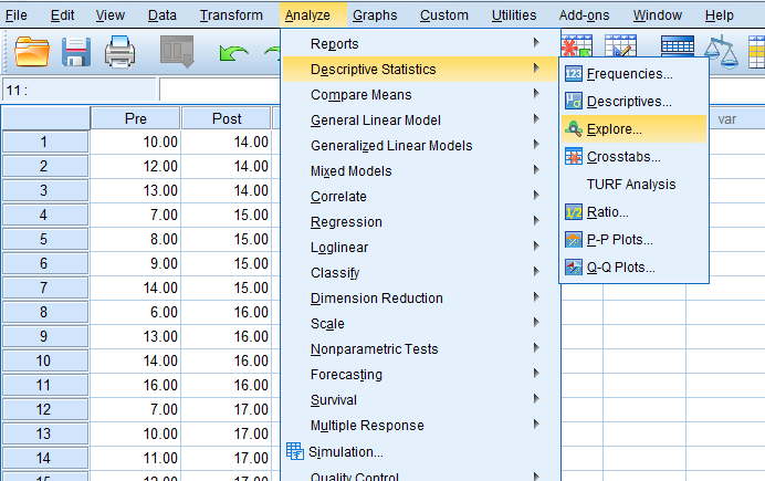
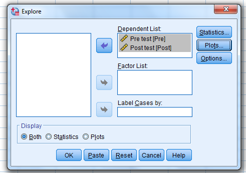
Click on “Analyze”…“Descriptive Statistics”…“Explore.”

When this pop-up pops up…

Select both the pre-test and post-test…move them…to the “Dependent List” box

…and then click on “Statistics.”

When this pop-up pops up…

Unselect “Outliers”…unselect “Percentiles”

…make sure that “Descriptives” are selected

…and then click “Continue.”

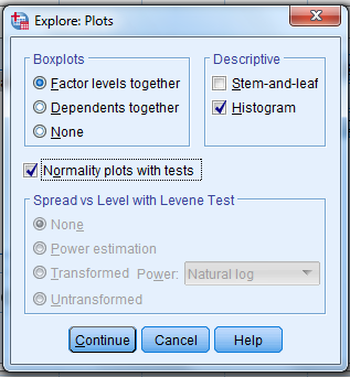
Then, click on “Plots.”

When this pop-up pops up…

Unselect “Stem-and-leaf”…select “Histogram”…select “Normality plots with tests”

…click “Continue”

…and click “OK.”

On the line for “Skewness”…use a calculator and divide the “Statistic” by the “Std. Error”

…which in this example is .156 / .246.

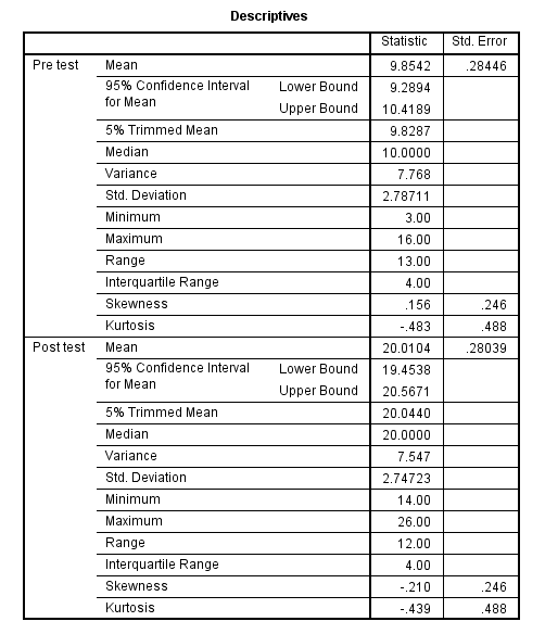
If the calculated value is within -1.96 to +1.96, then the variable is within the acceptable range for skewness.

Repeat this calculation for the statistic and std. error of the kurtosis. If the calculated value is within -1.96 to +1.96, then the variable is within the acceptable range for kurtosis.

Make sure to make these calculations for both the pre-test and the post-test.

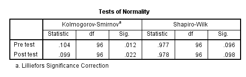
Look to see if the pre-test and post-test have “Shapiro-Wilk” “Sig.” values that are each > .05. If so, then the dependent variable is normally distributed and it meets the assumption of normal distribution. Make a note as to whether or not the assumption was met.

Inspect the histograms to see if the pre-test and post-test look approximately normally distributed. Make a note of this.

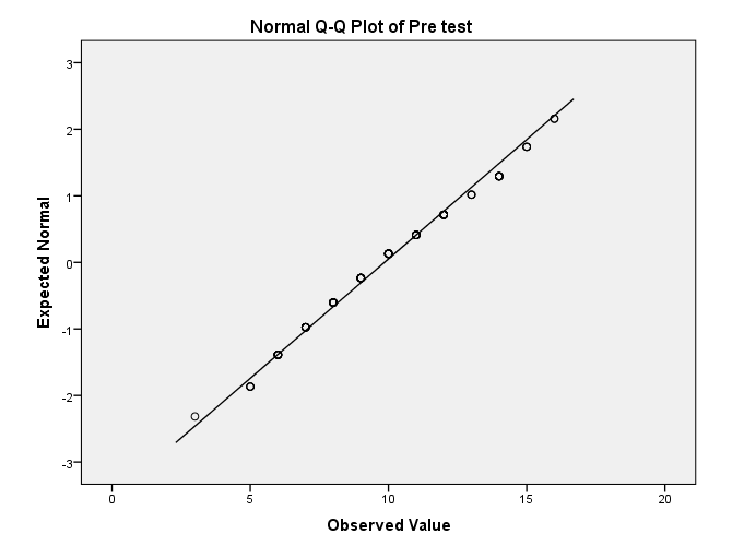
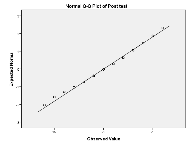
Inspect the “Normal Q-Q Plot” for the pre-test and post-test and note if the dots are close to the line.

Inspect the box plots of the pre-test and post-test and note if the whiskers are symmetrical.

1. Since we have met all of the assumptions, we can run the paired samples t-test.

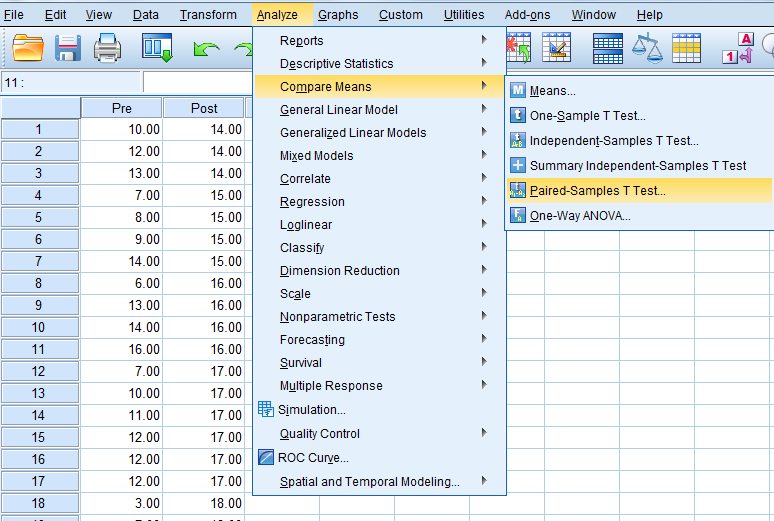
To do so, click “Analyze”…“Compare Means”…“Paired-Samples T Test.”

When this pop-up pops up…

Select the pre-test…and move it…over to the “Variable 1” box (NOTE: The pre-test must go in the Variable 1 box.)

…then, select the post-test…move it…over to the “Variable 2” box (NOTE: The post-test must go in the Variable 2 box.)

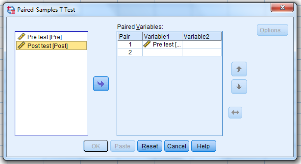
…and click “OK.”

In the output…

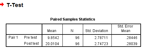
The “Paired Samples Statistics” table shows the means of the pre-test and post-test. On average, before watching the educational video, students washed their hands for 9.85 seconds. On average, after watching the video, students washed their hands for 20.01 seconds.

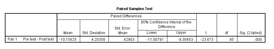
The “Paired Samples Test” table shows the difference of the means. If the “Sig.” value is < .05, then there is a statistically significant difference between the means of the pre-test and post-test. To calculate Cohen’s d for the effect size, we divide the mean difference by the standard deviation difference: 10.16/4.20 = 2.42 (this is a large effect!).

We can now report the paired samples t-test using the following template.

A paired samples t-test failed to reveal a statistically reliable difference between the mean number of older (M = 1.24, s = 1.26) and younger (M = 1.13, s = 1.20) siblings that the students have, t(44) = 0.377, p = .708, α = .05.

We performed a paired samples t-test in order to compare the difference of [variable being tested] among [description of the participants] before and after the [description of the intervention].

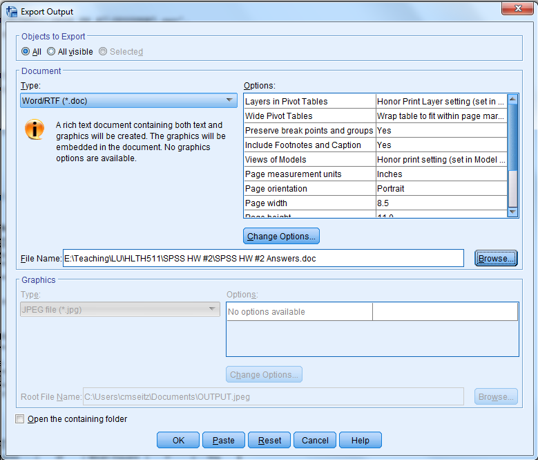
1. Finally, export your output to Word and submit it to Blackboard.

To export, click the export symbol

…click “Browse,” and then save your document with a name and location that you will remember.

Part 2

Follow the steps below to complete your SPSS homework assignment:

1. From Blackboard, download the SPSS HW #6-2 data file. Graduate student Q is interested in researching if an instructional handwashing video is effective in changing students’ ability to correctly perform all 5 steps of the CDC’s recommended handwashing procedure, which is measured as a yes/no index for each step of the procedure (1. Wet hands and apply soap; 2. Lather the back of the hands; 3. Lather between fingers; 4. Lather under the finger nails; 5. Lather for 20 seconds). In her study, Q conducted a pre-test. She had a group of student participants wash their hands at a sink, and she recorded whether or not each step was correctly performed each step. Based on how well the students washed their hands according to the 5 steps, students were given an index score grade of 0–5. Next, Q played the instructional handwashing video for them. Then, Q conducted a post-test by observing and recording the students’ ability to correctly perform each step of the handwashing procedure.

Before we can begin Wilcoxon Signed Ranks Test analysis, there are several assumptions we need to test for:

1. Measurement of variables (2 categorical/dependent [same people for pre/post test] groups; DV is ordinal or interval/ratio…if interval/ratio the distribution should not be normally distributed)

1. We have met the first assumption because we know that we have 2 categorical groups that are the exact same people for the pre-test and post-test and because we know that the DV is ordinal since it is measured as a 0–5 point scale.

1. Now, let’s run the analysis.

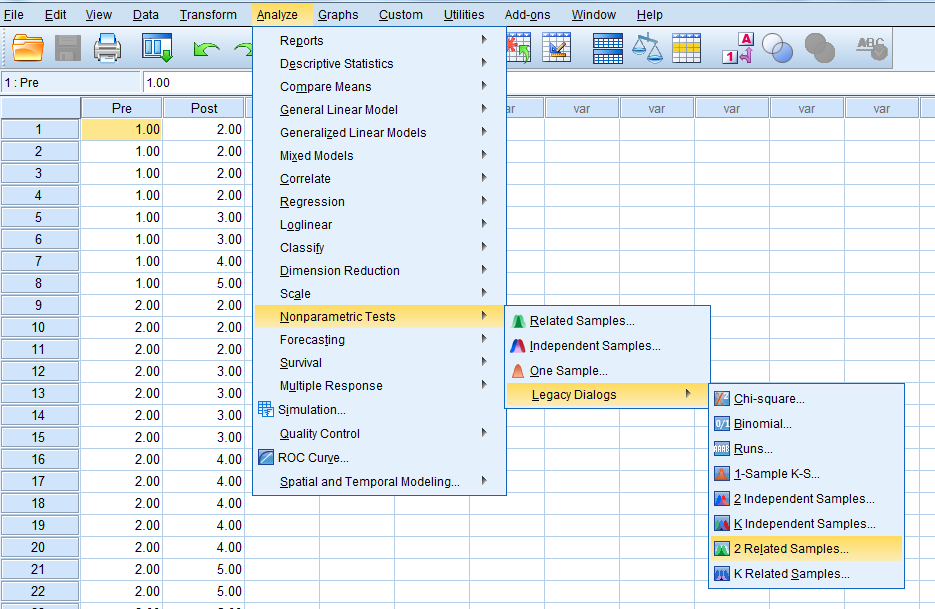
Click on “Analyze” … “Nonparametric Tests”…“Legacy Dialogs”…“2 Related Samples.”

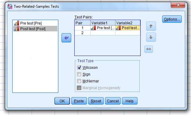
Select the pre-test variable…and move it…to the “Variable 1” box.

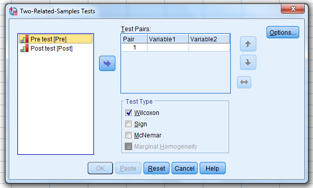
Then, select the post-test variable…and move it…to the “Variable 2” box.

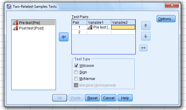
Make sure that “Wilcoxon” is selected and click “OK.”

We will also need to analyze the median of the pre-test and post-test.

Click “Analyze”…“Descriptive Statistics”…“Frequencies.”

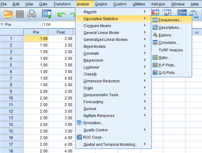
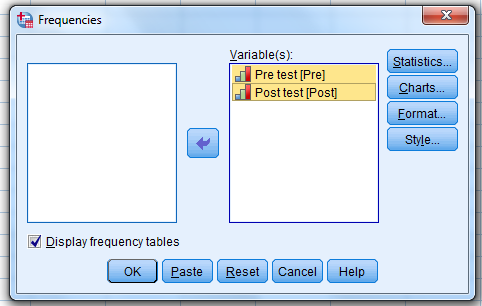
Select both the pre-test and the post-test…move them…to the “Variable(s)” box

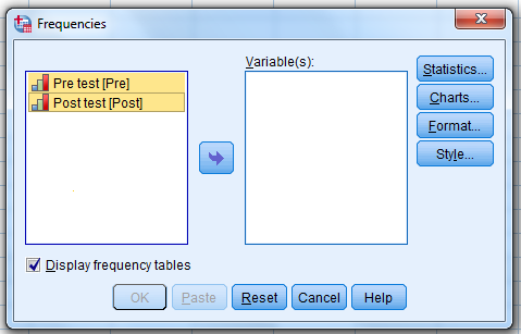
…and then click “Statistics.”

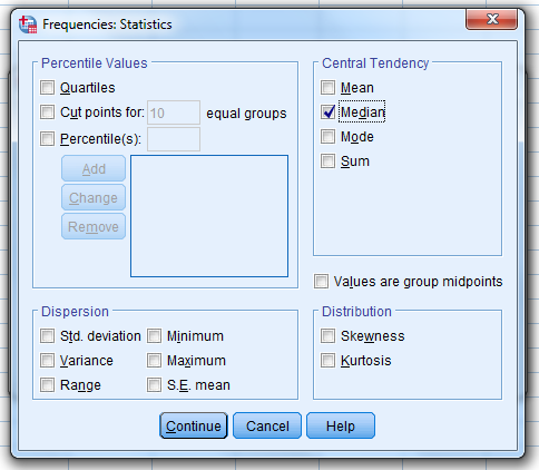
When this pop-up pops up…

Select “Median”…and click “Continue.”

1. Click OK

2. Finally, export your output to Word and submit it to Blackboard.

To export, click the export symbol

…click “Browse,” and then save your document with a name and location that you will remember.

Part 3

Follow the steps below to complete your SPSS homework assignment:

1. From Blackboard, download the SPSS HW #6-3 data file. Dr. F is interested in researching if there is a difference between male and female college students’ knowledge of the correct amount of time to wash their hands according to the CDC (which is 20 seconds). Dr. F has 2 groups of people (male and female) who are categorized into two groups (correct knowledge of handwashing seconds and incorrect knowledge of handwashing seconds).

Before we can begin the chi-square test of independence, there are a few assumptions we need to test for:

1. Both categorical V1 and V2 are nominal or ordinal

2. Both V1 and V2 are independent

1. We have met these assumptions because we know that we have 2 categorical groups measured as nominal/ordinal and the people are different people.

1. Let’s run the analysis…

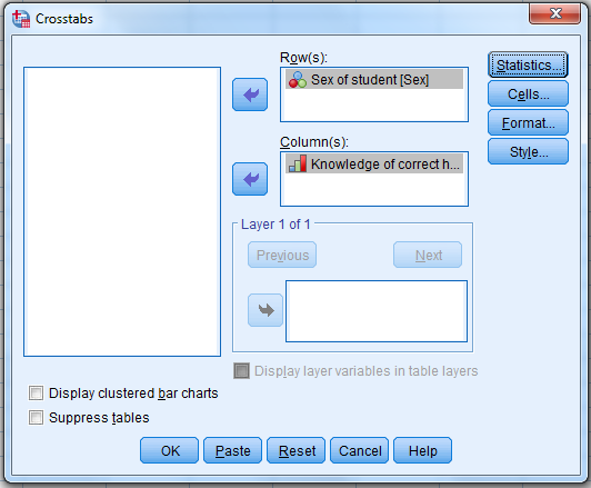
Click on “Analyze”…“Descriptive Statistics”…“Crosstabs”

When this pop-up pops up…

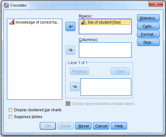
Select the independent variable…and move it … to the “Row(s)” box.

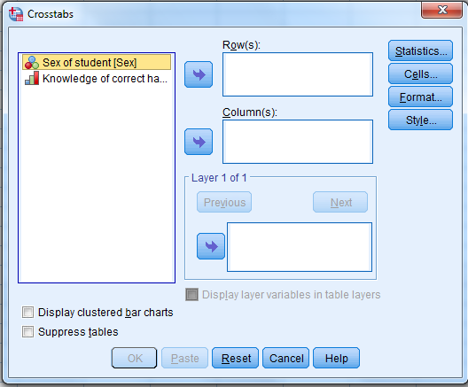
Select the dependent variable…move it…to the “Column(s)” box

…and then click on “Statistics.”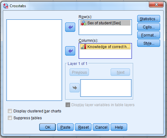

When this pop-up pops up…

Click on “Chi-square”…“Phi and Cramer’s V”…“Risk”

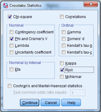
…and then click on “Continue.”

Click on “OK.”

Look at your output…

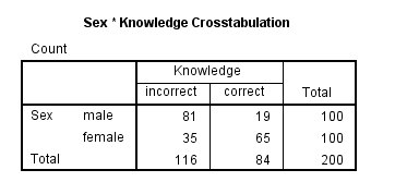
The “crosstabulation” table shows the frequency of each group of people for each variable. In the example below, there are: 81 males who fall within the “incorrect” handwashing knowledge, 19 males who have “correct” handwashing knowledge, 35 females who fall within the “incorrect” handwashing knowledge, 65 females who have “correct” handwashing knowledge. We want to make sure that there are at least 5 people in each category.

This gives a picture of what proportion of people fall within each category.

The “Chi-Square Tests” table shows us the Pearson chi-square value and if it is statistically significant. If this value is less than .05, it is significant.

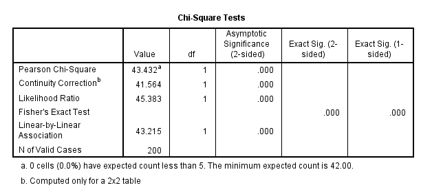
If we had a category that had less than 5 people, then we would look at the values that would appear in the “Fisher’s Exact Test” row.

The “Symmetric Measures” table contains the “Phi” value. This value is the effect size of doing a 2 x 2 chi-square test of independence.

For Phi, the rule of thumb is that a small effect is 0.1, a medium effect is 0.3, and large effect is 0.5.

Finally, check out the “risk estimate” table. This table contains the odds ratio.

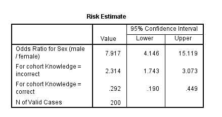
The odds ratio value says that the top row group is ____ times more likely than the bottom row group to experience the variable in the first column

This means that males are 7.92 times more likely than females to have incorrect knowledge about how many seconds are recommended for proper handwashing.

Or, we could switch the groups of the rows and columns and use the same odds ratio. This means that females are 7.92 times more likely than males to have correct knowledge.

If we take 1 divided by the odds ratio, we can make other statements that involve switching the rows and columns. So, 1/7.92 = 0.126.

This means that males are 0.126 times more likely than females to have correct knowledge.

Or, this means that females are 0.126 times more likely than males to have incorrect knowledge.

The odds ratios that are less than 1 do not make much sense, which is why only odds ratios that are greater than 1 are reported.

Below is an example of how to write up the results of the analysis above:

Remember the following format for reporting results and use this format when reporting results in the research project later in the course.

A chi-square test of independence was performed in order to compare the association of correct/incorrect knowledge between males/females. There was a statistically significant relationship between knowledge and gender χ2(1, N =200) -43.432, p < 0.05, φ = .466. According to the odds ratio, the odds of males having incorrect knowledge were 7.917 times greater than females.

1. Finally, export your output to Word and submit it to Blackboard.
   
   

To export, click the export symbol

…click “Browse,” and then save your document with a name and location that you will remember.