Master of Business Administration - MBA Semester 2 MB0045 - Financial Management - 4 Credits (Book ID: B1134) Assignment Set- 1 (60 Marks) Note: Each...
Master of Business Administration - MBA Semester 2
MB0045 – Financial Management - 4 Credits
(Book ID: B1134) Assignment Set- 1 (60 Marks)
Note: Each question carries 10 marks. Answer all the questions.
Q.1 What are the 4 finance decisions taken by a finance manager.
Q.2 What are the factors that affect the financial plan of a company?
Q.3 Show the relationship between required rate of return and coupon rate on the value of a bond.
Q.4 Discuss the implication of financial leverage for a firm.
Q.5 The cash flows associated with a project are given below:
Year Cash flow
0 (100,000)
1 25000
2 40000
3 50000
4 40000
5 30000
Calculate the a) payback period.
b) Benefit cost ratio for 10% cost of capital
Q6. A company’s earnings and dividends are growing at the rate of 18% pa. The growth rate is expected to continue for 4 years. After 4 years, from year 5 onwards, the growth rate will be 6% forever. If the dividend per share last year was Rs. 2 and the investors required rate of return is 10% pa, what is the intrinsic price per share or the worth of one share.
[Type text] [Type text] Nov 2010
Q.1 What are the 4 finance decisions taken by a finance manager ? Ans. Modern approach of financial management provides a conceptual and analytical framework for financial decision making. According to this approach there are 4 major decision areas that confront the Finance Manager these are:-
1. Investment Decisions 2. Financing Decisions 3. Dividend Decisions 4. Financial Analysis, Planning and Control Decisions
[A] Investment Decisions-: Investment decisions are made by investors and investment managers.
Investors commonly perform investment analysis by making use of fundamental analysis, technical analysis, screeners and gut feel.
Investment decisions are often supported by decision tools. The portfolio theory is often applied to help the investor achieve a satisfactory return compared to the risk taken.
[B] Financing Decisions-: What are the three types of financial management decisions? For each type of decision, give an example of a business transaction that would be relevant.
• There are three types of financial management decisions: Capital budgeting, Capital structure, and Working capital management.
• Capital budgeting is the process of planning and managing a firm's long-term investments. The key to capital budgeting is size, timing, and risk of future cash flows is the essence of capital budgeting. For example, yesterday I received a call from our manager over our Sand & Gravel Operations. He is looking into buying a new crusher (to crush stone into gravel and sand). I helped him today evaluate the return on investment for this opportunity. It quite a lot of work, but we determined that buying the new crusher would bring in 60,000 more tons of production/sales within the 1st year of owning the machine.
• Capital Structure refers to the
[C] Dividend Decisions-:The Dividend Decision is a decision made by the directors of a company. It relates to the amount and timing of any cash payments made to the company's stockholders. The decision is an important one for the firm as it may influence its capital structure and stock price. In addition, the decision may determine the amount of taxation that stockholders pay.
There are three main factors that may influence a firm's dividend decision:
Free-cash flow
Dividend clienteles
Information signalling
Under this theory, the dividend decision is very simple. The firm simply pays out, as dividends, any cash that is surplus after it invests in all available positive net present value projects.
A key criticism of this theory is that it does not explain the observed dividend policies of real-world companies. Most companies pay relatively consistent dividends from one year to the next and managers tend to prefer to pay a steadily increasing dividend rather than paying a dividend that fluctuates dramatically from one year to the next. These criticisms have led to the development of other models that seek to explain the dividend decision.
Dividend clienteles-: A particular pattern of dividend payments may suit one type of stock holder more than another. A retiree may prefer to invest in a firm that provides a consistently high dividend yield, whereas a person with a high income from employment may prefer to avoid dividends due to their high marginal tax rate on income. If clienteles exist for particular patterns of dividend payments, a firm may be able to maximise its stock price and minimise its cost of capital by catering to a particular clientele. This model may help to explain the relatively consistent dividend policies followed by most listed companies.
A key criticism of the idea of dividend clienteles is that investors do not need to rely upon the firm to provide the pattern of cash flows that they desire. An investor who would like to receive some cash from their investment always has the option of selling a portion of their holding. This argument is even more cogent in recent times, with the advent of very low-cost discount stockbrokers. It remains possible that there are taxation-based clienteles for certain types of dividend policies.
[D] Financial Analysis, Planning and Control Decisions-: Management has been defined as “the art of asking significant questions.” The same applies to financial analysis, planning and control, which should be targeted toward finding meaningful answers to these significant questions—whether or not the results are fully quantifiable.
This seminar not only presents the key financial tools generally used, but also explains the broader context of how and where they are applied to obtain meaningful answers. It provides a conceptual backdrop both for the financial/economic dimensions of systematic business management and for understanding the nature of financial statements, analyzing data, planning and controlling
Seminar Objectives-:The seminar provides delegates with the tools required to find better answers to questions such as: * What is the exact nature and scope of the issue to be analyzed? * Which specific variables, relationships, and trends are likely to be helpful in analyzing the issue? * Are there possible ways to obtain a quick “ballpark” estimate of the likely result? * How precise an answer is necessary in relation to the importance of the issue itself? * How reliable are the available data, and how is this uncertainty likely to affect the range of results?
* Are the input data to be used expressed in cash flow terms—essential for economic analysis—or are they to be applied within an accounting framework to test only the financial implications of a decision? What limitations are inherent in the tools to be applied, and how will these affect the range of results obtained? * How important are qualitative judgments in the context of the issue, and what is the ranking of their significance?
Who Should Attend? This seminar is a ‘must’ for Chief Financial Officers, Financial Controllers, Finance Executives, Accountants, Treasurers, Corporate Planning and Business Development Executives and Sales and Marketing Professionals.
Middle and junior personnel will also find this seminar highly useful in their career advancement. All participants will be able to offer their input, based on their individual experiences, and will find the seminar a forum for upgrading and enhancing their understanding of best corporate practices in the areas examined.
Competencies Emphasised-: * Obtaining the relevant information, given the context of the situation * Choosing the most appropriate tools * Knowing the strengths and limitations of the available tools * Viewing all analysis, planning and control decisions in the context of their impact on * shareholder value
Personal Impact-: Delegates will acquire the ability, when involved in decisions about business investment, operations, or financing, to choose the most appropriate tools from the wide variety of analytical techniques available to generate quantitative answers. Selecting the appropriate tools from these choices is clearly an important part of the analytical task. Yet, experience has shown again and again that first developing a proper perspective for the problem or issue is just as important as the choice of the tools themselves.
Organisational Impact-: This seminar provides an integrated conceptual backdrop both for the financial/economic dimensions of systematic business management and for understanding the nature of financial statements.
All the topics on the seminar are viewed in the context of creating shareholder value—a fundamental concept that is consolidated on the final day of the seminar.
Training Methodology-: The training methodology combines lectures, discussions, group exercises and individual exercises. Delegates will gain both a theoretical and a practical knowledge of the topics covered. The emphasis is on the practical application of the topics and as a result delegates will return to the workplace with both the ability and the confidence to apply the techniques learned, in carrying out their duties. All delegates will receive a comprehensive set of notes to take back to the workplace, which will serve as a useful source of reference in the future. In addition, all delegates will receive a CD-ROM disk containing additional reference material and Excel templates, related to the seminar.
Seminar Outline-:
Day 1 – The Challenge of Financial/Economic Decision-making * The practice of financial/economic analysis * The value-creating company * A dynamic perspective of business * What information and data to use * The nature of financial statements * The context of financial analysis
Day 2 – Assessment of Business Performance * Ratio analysis and performance * Management’s point of view * Owners’ point of view * Lenders’ point of view * Ratios as a system * Integration of financial performance analysis * Some special issues
Day 3 – Projection of Financial Requirements * Interrelationship of financial projections * Operating budgets * Standard costing and variance analysis * Cash forecasts/budgets * Sensitivity analysis * Dynamics and growth of the business system * Operating leverage * Financial growth plans * Financial modelling
Day 4 – Analysis of Investment Decisions * Applying time-adjusted measures * Strategic perspective * Economic value added (EVA) and net present value (NPV) * Refinements of investment analysis * Equivalent annual cost (EAC) * Modified internal rate of return (MIRR) * Dealing with risk and changing circumstances
Day 5 – Valuation and Business Performance * Managing for shareholder value * Shareholder value creation in perspective * Evolution of value-based methodologies * Creating value in restructuring and combinations * Financial strategy in acquisitions * Business valuation * Business restructuring and reorganisations * Management buy-outs and management buy-ins
Q. 2 What are the factors that affect the financial plan of a company ?
Ans Nature of industry: The nature of the industry in which the company is performing is a major factor which affects financial plans. A labour- intensive industry requires less capital than a capital-intensive industry.
Status of the company in the industry: The status of the company is a factor which has to be considered while drawing a financial plan. If the company is a well-recognized and a reputed one, it will have no problems in raising finance at short notices. But on the other hand, if the company is a new entrant into the field, it will need time to establish itself and therefore raising money is slightly difficult, especially so if the company wants to go public. New firms may find it easier and better to take loans and function rather than going public.
Alternative sources of finance: The Finance Manager will assess the alternative sources of funds and get the cheapest source of funds. He should also verify the conditions attached to the funds he procures, that are the contractual restrictions placed by the lenders.
Attitude of management towards control: If the management wants to have control over the firm, it may not go in for the equity form of finance for control vests with equity shareholders and it gets diluted with every new issue of equity shares. Such companies prefer to raise additional amounts by debenture issue or bond issue.
Extent of working capital requirements: The Finance Manager formulates his plan considering the short and long term financial needs of the firm. Short term funds required to finance working capital needs are to be procured through short term sources only. It is always a prudent policy to use short term avenues for short term requirements and long term needs can be funded by the issue of shares and debentures.
Capital structure: Capital of a firm has two components – debt and equity. The proportion of these should be so decided that the company gets the advantage of leverage. Running the company with loans and debentures will certainly help equity shareholders to get more income but the company is also functioning under a great risk.
Flexibility: This is one important factor that should be kept in mind while planning. The financial plan should be flexible enough to adjust to the needs of the changing conditions. There should be flexibility to raise the amount from any source and similarly the repayments may be done any time the company has excess funds. The firm should also have the flexibility of substituting one form of financing with another if the need arises.
Government policy: with regard to financial controls, statutory provisions and controls should be considered. The SEBI guidelines should be strictly adhered to wherever applicable and necessary permissions from concerned authorities should be taken if necessary.
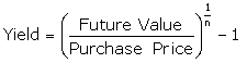
Q.3 Show the relationship between required rate of return and coupon rate on the value of a bond ? Ans. Advanced Bond Concepts: Yield and Bond Price-: In the last section of this tutorial, we touched on the concept of required yield. In this section we'll explain what this means and take a closer look into how various yields are calculated. The general definition of yield is the return an investor will receive by holding a bond to maturity. So if you want to know what your bond investment will earn, you should know how to calculate yield. Required yield, on the other hand, is the yield or return a bond must offer in order for it to be worthwhile for the investor. The required yield of a bond is usually the yield offered by other plain vanilla bonds that are currently offered in the market and have similar credit quality and maturity. Once an investor has decided on the required yield, he or she must calculate the yield of a bond he or she wants to buy. Let's proceed and examine these calculations.
Calculating Current Yield
A simple yield calculation that is often used to calculate the yield on both bonds and the dividend yield for stocks is the current yield. The current yield calculates the percentage return that the annual coupon payment provides the investor. In other words, this yield calculates what percentage the actual dollar coupon payment is of the price the investor pays for the bond. The multiplication by 100 in the formulas below converts the decimal into a percentage, allowing us to see the percentage return:
|
|
So, if you purchased a bond with a par value of $100 for $95.92 and it paid a coupon rate of 5%, this is how you'd calculate its current yield:
|
|
Notice how this calculation does not include any capital gains or losses the investor would make if the bond were bought at a discount or premium. Because the comparison of the bond price to its par value is a factor that affects the actual current yield, the above formula would give a slightly inaccurate answer - unless of course the investor pays par value for the bond. To correct this, investors can modify the current yield formula by adding the result of the current yield to the gain or loss the price gives the investor: [(Par Value – Bond Price)/Years to Maturity]. The modified current yield formula then takes into account the discount or premium at which the investor bought the bond. This is the full calculation:
|
|
Let's re-calculate the yield of the bond in our first example, which matures in 30 months and has a coupon payment of $5:
|
|
The adjusted current yield of 6.84% is higher than the current yield of 5.21% because the bond's discounted price ($95.92 instead of $100) gives the investor more of a gain on the investment.
One thing to note, however, is whether you buy the bond between coupon payments. If you do, remember to use the dirty price in place of the market price in the above equation. The dirty price is what you will actually pay for the bond, but usually the figure quoted in U.S. markets is the clean price.
Now we must also account for other factors such as the coupon payment for a zero-coupon bond, which has only one coupon payment. For such a bond, the yield calculation would be as follows:
|
|
If we were considering a zero-coupon bond that has a future value of $1,000 that matures in two years and can be currently purchased for $925, we would calculate its current yield with the following formula:
|
|

Calculating Yield to Maturity
The current yield calculation we learned above shows us the return the annual coupon payment gives the investor, but this percentage does not take into account the time value of money or, more specifically, the present value of the coupon payments the investor will receive in the future. For this reason, when investors and analysts refer to yield, they are most often referring to the yield to maturity (YTM), which is the interest rate by which the present values of all the future cash flows are equal to the bond's price.
An easy way to think of YTM is to consider it the resulting interest rate the investor receives if he or she invests all of his or her cash flows (coupons payments) at a constant interest rate until the bond matures. YTM is the return the investor will receive from his or her entire investment. It is the return that an investor gains by receiving the present values of the coupon payments, the par value and capital gains in relation to the price that is paid.
The yield to maturity, however, is an interest rate that must be calculated through trial and error. Such a method of valuation is complicated and can be time consuming, so investors (whether professional or private) will typically use a financial calculator or program that is quickly able to run through the process of trial and error. If you don't have such a program, you can use an approximation method that does not require any serious mathematics.
To demonstrate this method, we first need to review the relationship between a bond's price and its yield. In general, as a bond's price increases, yield decreases. This relationship is measured using the price value of a basis point (PVBP). By taking into account factors such as the bond's coupon rate and credit rating, the PVBP measures the degree to which a bond's price will change when there is a 0.01% change in interest rates.
The charted relationship between bond price and required yield appears as a negative curve:
|
|

This is due to the fact that a bond's price will be higher when it pays a coupon that is higher than prevailing interest rates. As market interest rates increase, bond prices decrease.
The second concept we need to review is the basic price-yield properties of bonds:
| Premium bond: Coupon rate is greater than market interest rates. |
Thirdly, remember to think of YTM as the yield a bondholder receives if he or she reinvested all coupons received at a constant interest rate, which is the interest rate that we are solving for. If we were to add the present values of all future cash flows, we would end up with the market value or purchase price of the bond.
The calculation can be presented as:
|
|

OR
|
|

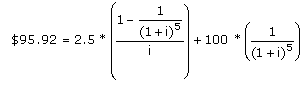
Example 1: You hold a bond whose par value is $100 but has a current yield of 5.21% because the bond is priced at $95.92. The bond matures in 30 months and pays a semi-annual coupon of 5%.
1. Determine the Cash Flows: Every six months you would receive a coupon payment of $2.50 (0.025*100). In total, you would receive five payments of $2.50, plus the future value of $100.
2. Plug the Known Amounts into the YTM Formula:
|
|
Remember that we are trying to find the semi-annual interest rate, as the bond pays the coupon semi-annually.
3. Guess and Check: Now for the tough part: solving for “i,” or the interest rate. Rather than pick random numbers, we can start by considering the relationship between bond price and yield. When a bond is priced at par, the interest rate is equal to the coupon rate. If the bond is priced above par (at a premium), the coupon rate is greater than the interest rate. In our case, the bond is priced at a discount from par, so the annual interest rate we are seeking (like the current yield) must be greater than the coupon rate of 5%. Now that we know this, we can calculate a number of bond prices by plugging various annual interest rates that are higher than 5% into the above formula. Here is a table of the bond prices that result from a few different interest rates:
|
|

Because our bond price is $95.92, our list shows that the interest rate we are solving for is between 6%, which gives a price of $95, and 7%, which gives a price of $98. Now that we have found a range between which the interest rate lies, we can make another table showing the prices that result from a series of interest rates that go up in increments of 0.1% instead of 1.0%. Below we see the bond prices that result from various interest rates that are between 6.0% and 7.0%:
|
|
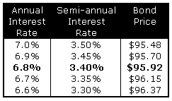
We see then that the present value of our bond (the price) is equal to $95.92 when we have an interest rate of 6.8%. If at this point we did not find that 6.8% gives us the exact price that we are paying for the bond, we would have to make another table that shows the interest rates in 0.01% increments. You can see why investors prefer to use special programs to narrow down the interest rates - the calculations required to find YTM can be quite numerous!
Calculating Yield for Callable and Puttable Bonds
Bonds with callable or puttable redemption features have additional yield calculations. A callable bond's valuations must account for the issuer's ability to call the bond on the call date and the puttable bond's valuation must include the buyer's ability to sell the bond at the pre-specified put date. The yield for callable bonds is referred to as yield-to-call, and the yield for puttable bonds is referred to as yield-to-put.
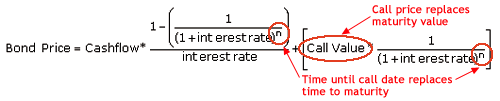
Yield to call (YTC) is the interest rate that investors would receive if they held the bond until the call date. The period until the first call is referred to as the call protection period. Yield to call is the rate that would make the bond's present value equal to the full price of the bond. Essentially, its calculation requires two simple modifications to the yield-to-maturity formula:
|
|
Note that European callable bonds can have multiple call dates and that a yield to call can be calculated for each.
Yield to put (YTP) is the interest rate that investors would receive if they held the bond until its put date. To calculate yield to put, the same modified equation for yield to call is used except the bond put price replaces the bond call value and the time until put date replaces the time until call date. For both callable and puttable bonds, astute investors will compute both yield and all yield-to-call/yield-to-put figures for a particular bond, and then use these figures to estimate the expected yield. The lowest yield calculated is known as yield to worst, which is commonly used by conservative investors when calculating their expected yield. Unfortunately, these yield figures do not account for bonds that are not redeemed or are sold prior to the call or put date. Now you know that the yield you receive from holding a bond will differ from its coupon rate because of fluctuations in bond price and from the reinvestment of coupon payments. In addition, you are now able to differentiate between current yield and yield to maturity. In our next section we will take a closer look at yield to maturity and how the YTMs for bonds are graphed to form the term structure of interest rates, or yield curve.
Q.4 Discuss the implication of financial leverage for a firm.? Ans-: In physics, leverage denotes the use of a lever and a small amount of force to lift a heavy object. Likewise in business, leverage refers to the use of a relatively small investment or a small amount of debt to achieve greater profits. That is, leverage is the use of assets and liabilities to boost profits while balancing the risks involved. There are two types of leverage, operating and financial. Operating leverage refers to the use of fixed costs in a company's earnings stream to magnify operating profits. Financial leverage, on the other hand, results from the use of debt and preferred stock to increase stockholder earnings. Although both types of leverage involve a certain amount of risk, they can bring about significant benefits with little investment when successfully implemented.
FINANCIAL LEVERAGE-: Financial leverage involves changes in shareholders' income in response to changes in operating profits, resulting from financing a company's assets with debt or preferred stock. Similar to operating leverage, financial leverage also can boost a company's returns, but it increases risk as well. Financial leverage is concerned with the relationship between operating profits and earnings per share. If a company is financed exclusively with common stock, a specific percentage change in operating profit will cause the
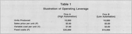 Table 1
Illustration Of Operating Leverage
| Firm A | Firm B | |
| Units Produced | 10,000 | 10,000 |
| Sales price per unit (P) | S5.00 | $5.00 |
| Variable cost per unit (V) | $1.00 | $3.00 |
| Fixed costs (F) | $35,000 | $15,000 |
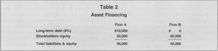 Table 2
Asset Financing
| Firm A | Firm B | |
| Long-term debt (8%) | $10,000 | $ 0 |
| Stockholders equity | 30,000 | 40,000 |
| Total liabilities & equity | 40,000 | 40,000 |
same percentage change in shareholder earnings. For example, a 5 percent increase in operating profit will result in a 5 percent increase in shareholder earnings. If a company is financed with debt or is "leveraged," however, its shareholder earnings will become more sensitive to changes in operating profit. Hence, a 5 percent increase in operating profits will result in a much higher increase in stockholder earnings. Nevertheless, financial leveraging makes companies equally susceptible to greater decreases in stockholder earnings if operating profits drop. For example, recall the two firms, A and B. At production levels of 10,000 widgets, they both had operating earnings (profits) of $5,000. In addition, assume that both firms have total assets of $40,000. Table 2 shows how the $40,000 of assets are financed for both firms. Firm A is financed with $10,000 of debt which carries an annual interest cost of 8 percent, and $30,000 of stockholders' equity (3,000 shares), firm B is financed entirely with $40,000 of stockholders' equity (4,000 shares). Firm A is leveraged and uses some debt to finance its assets, which can increase earnings per share but also risk. Table 3 shows the results of financial leverage on the firm's earnings. Panel A shows that as a result of the $800 interest expense from the debt ($10,000 X. 08 = $800), firm A's earnings per share are lower than firm B's. Because firm A is financially leveraged, however, an increase in profits will result in a greater increase in stock earnings. Panel B shows the results of a 10 percent increase in profits for both firms. Firm A's stockholder earnings increased from $0.84 to $0.94, an 11.9 percent increase, while firm B's stockholder earnings increased from $0.75 to $0.825, or 10 percent, the same as the increase in profits.
 Table 3
Illustration of Financial Leverage
| Panel A Operating Income = $5,000 | ||
| Firm A | Firm B | |
| Operating income (EBIT) | $5,000 | $5,000 |
| Less: interest expense | (800) | (0) |
| Earnings before taxes (EBT) | 4,200 | 5,000 |
| Less: taxes (40%) | (1,680) | (2,000) |
| Net profits after taxes (NPAT) | 2,520 | 3,000 |
| Divided by number of shares | 3000 | 4000 |
| Earnings per share (EPS) | $0.84 | $0.75 |
| Panel B Operating Income = $5,500 | ||
| Firm A | Firm B | |
| Operating income (EBIT) | $5,500 | $5,500 |
| Less: interest expense | (800) | (0) |
| Earnings before taxes (EBT) | 4,700 | 5,500 |
| Less: taxes (40%) | (1,880) | (2,200) |
| Net profits after taxes (NPAT) | 2,820 | 3,300 |
| Divided by number of shares | 3000 | 4000 |
| Earnings per share (EPS) | $0.94 | $0,825 |
| Increase in EPS | $0.10 | $0.94 |
| Percentage increase in EPS | 11.90% | 10.0% |
Companies with significant amounts of debt in contrast with their assets are referred to as being highly leveraged and their shareholder earnings are more unpredictable than those for companies with less debt. Lenders and financial analysts often measure a company's degree of financial leverage using the ratio of interest payments to operating profit. From the perspective of shareholders, financing using debt is the riskiest, because companies must make interest and principal payments on debt as part of their contract with their lenders, but they need not pay preferred stock dividends if their earnings are low. Nevertheless, financing with preferred stock will have the same kind of leveraging effect as debt financing as illustrated above. Firms that use financial leverage run the risk that their operating income will be insufficient to cover the fixed charges on debt and/or preferred stock financing. Financial leverage can become especially burdensome during an economic downturn. Even if a company has sufficient earnings to cover its fixed financial costs, its returns could be decreased during economically difficult times due to shareholders' residual claims to dividends. Generally, if a company's return on assets (profits. total assets) is greater than the pretax cost of debt (interest percentage), the financial leverage effect will be favorable. The opposite, of course, is also true: if a company's return on assets is less than its interest cost of debt, the financial leverage effect will decrease the returns to the common shareholders.
TOTAL LEVERAGE-: The two types of leverage explored so far can be combined into an overall measure of leverage called total leverage. Recall that operating leverage is concerned with the relationship between sales and operating profits, and financial leverage is concerned with the relationship between profits and earnings per share. Total leverage is therefore concerned with the relationship between sales and earnings per share. Specifically, it is concerned with the sensitivity of earnings to a given change in sales. The degree of total leverage is defined as the percentage change in stockholder earnings for a given change in sales, and it can be calculated by multiplying a company's degree of operating leverage by its degree of financial leverage. Consequently, a company with little operating leverage can attain a high degree of total leverage by using a relatively high amount of debt.
IMPLICATIONS-:Total risk can be divided into two parts: business risk and financial risk. Business risk refers to the stability of a company's assets if it uses no debt or preferred stock financing. Business risk stems from the unpredictable nature of doing business, i.e., the unpredictability of consumer demand for products and services. As a result, it also involves the uncertainty of long-term profitability. When a company uses debt or preferred stock financing, additional risk—financial risk—is placed on the company's common shareholders. They demand a higher expected return for assuming this additional risk, which in turn, raises a company's costs. Consequently, companies with high degrees of business risk tend to be financed with relatively low amounts of debt. The opposite also holds: companies with low amounts of business risk can afford to use more debt financing while keeping total risk at tolerable levels. Moreover, using debt as leverage is a successful tool during periods of inflation. Debt fails, however, to provide leverage during periods of deflation, such as the period during the late 1990s brought on by the Asian financial crisis.
FURTHER READING:- Brigham, Eugene F. Fundamentals of Financial Management. Fort Worth, TX: Dryden Press, 1995."Choosing the Right Mixture." Economist, 27 February 1999, 71. Dugan, Michael T., and Keith A. Shriver. "An Empirical Comparison of Alternative Methods for Estimating the Degree of Operating Leverage." Financial Review, May 1992, 309-21. Jaedicke, Robert K., and Alexander A. Robichek. "Cost-Volume-Profit Analysis under Conditions of Uncertainty." Accounting Review, October 1964, 917-26. Krefetz, Gerald. Leverage: The Key to Multiplying Money. New York: Wiley, 1988. Shalit, Sol S. "On the Mathematics of Financial Leverage." Financial Management, spring 1975, 57-66.
Q.5 The cash flows associated with a project are given below:
Year Cash flow
0 (100,000)
1 25000
2 40000
3 50000
4 40000
5 30000
Calculate the a) payback period.
b) Benefit cost ratio for 10% cost of capital
Ans.
[a] Payback period:
The cash flows and the cumulative cash flows of the projects is shown under in table
Table Cash flows and cumulative cash flows
Year Project Cash flows (Rs.) Cumulative Cash flows
1 25,000 25,000
2 40,000 65,000
3 50,000 115,000
4 40,000 155,000
5 30,000 185,000
From the cumulative cash flow column the initial cash outlay of Rs. 1,00,000 lies between 2nd year and 3rd year in respect of project. Therefore, payback period for project is:
= 2.54 years
Pay-back period for project B is 2.54 years.
b) Benefit cost ratio for 10% cost of capital
Table: Present Value (PV) of Cash inflows
Year Cash in flows PV factor at 15% PV of Cash in flows
1 25,000 0.909 22,725
2 40,000 0.826 33,040
3 50,000 0.751 37,550
4 40,000 0.683 27,320
5 30,000 0.621 18,630
PV of Cash inflow = 139,265
Initial Cash out lay = 1,00,000
NPV = 39,265
Benefit cost ratio = PV of Cash inflow/Initial Cash outlay
Benefit cost ratio = 139,265/1,00,000
Benefit cost ratio = 1.39


