need help in Rstudio project
Project Final Deliverable
Overall Goals / Research HypothesisThe goal of my research is to analysis the dataset provided which contains the roughly 3 million tweets from the IRA (Internet Research Agency) and derive enough features from that dataset to be able to train a model to analyze and detect troll tweets. The dataset that is provided contains a four different main descriptions of twitter account categories:
- Right Trolls
- Left Trolls
- Hashtag Gamers
- Fearmongers
- News Feed
- Commercial
Each one of the categories has a distinct subset of attributes which can be closely linked to the words used in the tweet themselves. The only category that is a bit harder to predict would be the Hashtag gamers since those relied more on hashtag games such as #OffendEveryoneIn4Words or #WasteAMillionIn3Words. Due to this limitation, this study will focus on the Left Trolls and the Right Trolls as well as a combined database of them both to see if we can broadly classify using that. The Right and Left trolls tweeted out based on agendas to try and spur certain movements. This would mean that there should be many similarities between the tweets themselves which would give us enough data to create features based on the frequencies and other information.
The experiment will look at current day tweets and see if we can reasonably classify a tweet to not be a troll tweet. The problem with this will be that most of the troll tweets rely on a political agenda, so this may lead to false classifications on any tweets containing any form of political verbiage. To gather metrics on the dataset we will analyze the tweets themselves and look at the words used. This will lead to features being extracted based on the words used which will hopefully let the model determine troll tweets. The non-troll tweets will be gathered from a Kaggle dataset (https://www.kaggle.com/kazanova/sentiment140) that was used for sentiment analysis and those will be used in conjunction with our other dataset.
The original hypothesis we stated was aimed at classifying an individual tweet. While that did result in some success, the result, which we will discuss later, was not as satisfying. After taking a second look at the data a new hypothesis was drawn up, can we classify the account as a troll, not the individual tweet.
Previous / Relate ContributionsDue to this dataset not being a Kaggle study it does lead to some difficulty finding related studies and contributions to the dataset. Most of the analysis that has been done on the data is merely a look at what trends we see in the data but not much as far as machine learning applications. One of the articles that discussed the dataset looked at the dates of the tweets themselves and what dates were the most popular, not surprisingly enough they closely correlated with election time, roughly 350,000 retweets per week just before the election [2]. This dataset comes from twitter which utilizes hashtags to enforce topics of interest so one of the other data analysis aspects is to look at the hashtags themselves and see what ones were the most popular, sadly only 33% of the English tweets contained a hashtag. The data that author Kate Starbird displays shows that there was really no politically motivated hashtag till around number 9, MAGA, but do notice a few other ones at 13, 15, and 20. This shows that while the hashtags might not be the easiest way to define the dataset, it could be possible to do such. A tweet can however contain multiple hashtags in it, and this displays the links between certain tags, like #BlackLivesMatter and #BlackTwitter or #PoliceBrutality. Another anecdote of analysis is that a method of trolling is to routinely reply to tweets back and forth, this connection can also be analyzed to see if the troll accounts are collaborating, another defining feature.
Another analysis done by Clemson University looked at the specific categories within the dataset and tried to find defining characteristics among them. The themes of the tweets along with the hashtags used were described as sending “divisive messages about mainstream and moderate Republicans” [1]. These accounts would attack the mainstream targets and try to sow a thought of questionable credibility about the campaign. Another note realized that this category also contained some theme specific accounts, like one about the secession of Texas, which might skew some of the data. Most of the data however had identifying information. The Left trolls also fell into a similar boat with specific hashtags and attempting to undermine credibility of mainstream Democratic actors. One side note to that however is that the Left trolls did in fact seem to be supportive of Bernie Sanders prior to the election. The other categories did have some specific characteristics as well but those were not as defining as the Left and Right trolls.
While the data analysis provided from previous results does give us an insight in the dataset, it does not help with finding any adequate machine learning algorithms that have used the dataset. There are however other research projects that have looked at the sentiment analysis of tweets from other datasets like this one from Kaggle:
https://www.kaggle.com/kazanova/sentiment140 (aka our Truth Dataset)
This gives us a good idea of what kind of defining characteristic we could use. As well as how we will want to try to format our data. Sadly however our models are going for more of a classifier approach in an attempt to classify the tweet as a malicious troll or not, however we could perform sentiment analysis and see if that is a good feature of the troll tweet itself, I.E the sentiment of the troll tweets tends to trend in the negative side.
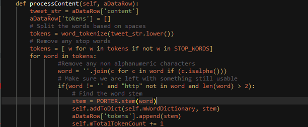
Features Selection / EngineeringSince we are going with a text analysis model, we need to attempt to extract features from the words themselves. This can give a few different features such as TF-IDF, Sentiment, Count Vectors, Word Embedding, and Topic Models. Before any of those can be considered however, we must first get the content into a usable format and narrow the words down, we can do this by stemming and remove common stop words as well as filtering words with a length larger than two. We do so here:
After we have accomplished this step, we now have data we can work with to extract some features. Since the dataset is very large, 3 million tweets and my computer only has 8 GB of ram I will use one CSV into the python code to train / test the feature extraction. There are three categories that we will look at in depth, Right Trolls, Left Trolls, and a Combined model which contains all the tweets in the dataset. We can easily filter based on the category in the CSV file provided and then generate our own CSV files with just the category that the specific model cares about.
After generating and the tokens, we then can analyze word frequencies from those tweets themselves. This can easily be visualized using the WordCloud library in python:
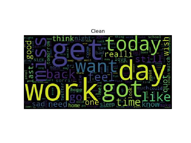
NOTE: The clean data was only 25k tweets to get this plot since it was chewing up my RAM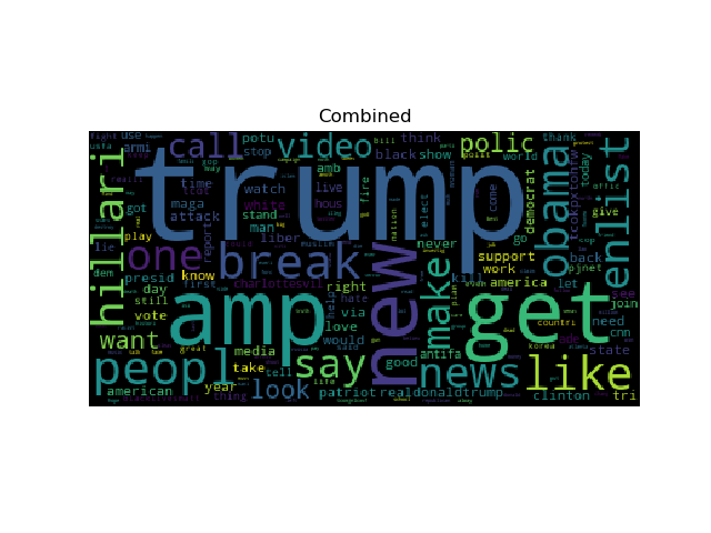
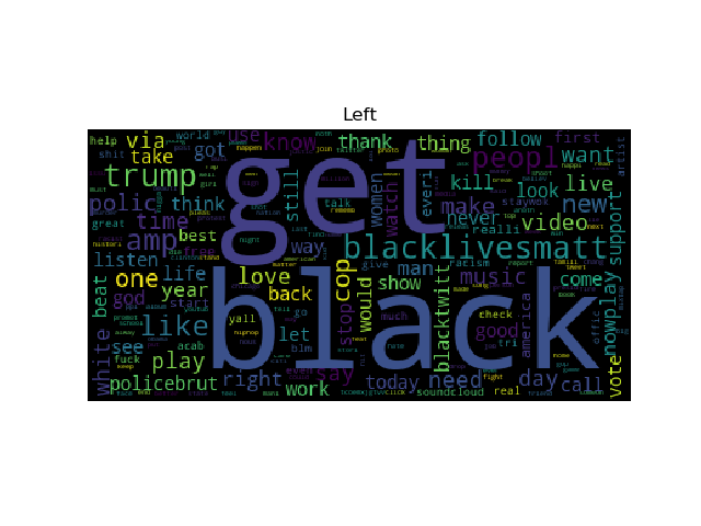
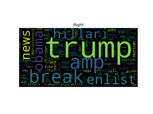
Due to the stemming of words we see some clipping of letters that shouldn’t be, but we see the important trends here starting to show up. The Right Troll displays more frequent words like trump, hillary, maga and Obama while the Left troll displays words like black, blacklivesmatter, and policebrutality. Due to the nature of twitter some words get combined because they were used in repeated hashtags, like what we see with blacklivesmatter, but we should see similar trends in the input data since that is a defined behavior. Another thing to note is how the clean data wordCloud looks very normal, there was not many trends in that data, but the word counts look like everyday words, that’s the trend we would want from that data.
Now that we have tokens vectorized and word frequencies sorted out into a dictionary corpus we can look at extracting some valuable features. TF-IDF, Term frequency and Inverse Document Frequency, help us represent the relative importance of a term within the document itself and within the entire corpus. Since we want to look at classifying an unsupervised dataset the data will need to be somewhat combined into the same corpus but still kept separate when we calculate TF-IDF, this is because certain words show up more frequently in the Left Model and other ones more frequently in the Right Model. After running the following code to generate TF-IDF based on a tokenized tweet and then re-formatting them to the correct format for the sklearn vectorizer we can then train a KMeans Cluster, Naïve Bayes, SVM or whatever other models we would like.
With our modified hypothesis the TF-IDF is instead extended out to the all the tweets from an induvial account rather than the single tweet. By making the ‘document’ for the TF-IDF larger, we now have a larger amount of words for each document, which means the that individual document frequencies are larger now too. This will affect how much a word means to a document but hopefully by modifying the dataset like such, it will mean we have more to classify with.
Another avenue for a feature to explore is the sentiment of the statement itself. Calculating the sentiment can give us another feature to look at however when it comes to classifying based on the content of a text it does not buy us much. Since we are trying to look at a tweet and say whether or not it is a troll tweet we do not care what the sentiment was but rather how closely related the text of the tweet is compared to the text in the tweets from our dataset, which we can achieve using TF-IDF.
Sentiment analysis itself is also good because it allows us to analyze the dataset before we start to use it in our classifiers. While we know we have two individual datasets and we can mark them using our own target, it is good to know how the sentiment is picked up in each one. In theory we would think that the troll tweets would mostly contain a negative sentiment while the casual tweets would mostly contain a positive sentiment. With our original hypothesis we can see that the sentiment itself is very much all over the place.
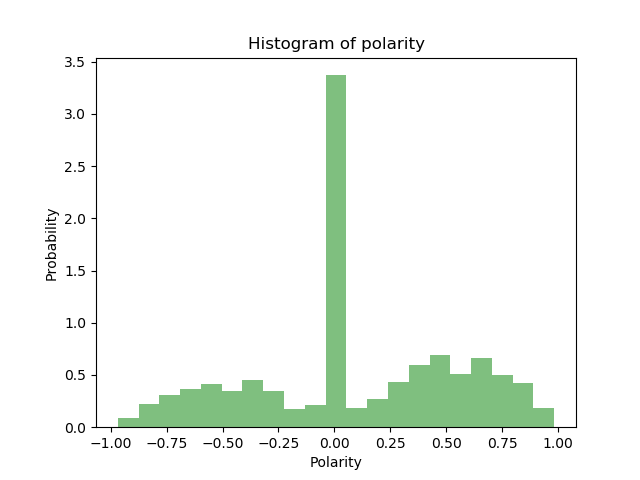
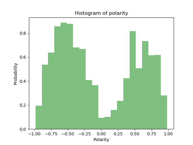
We can see in the above graph that the dataset is having a lot of tweets being flagged as a neutral polarity. If we wanted to further clean the dataset, a method could be done to prune out the neutral flagged tweets, this would result in leaving us with tweets only containing a positive polarity above some threshold and a negative polarity below some threshold. Originally it was done without using polarity to check against the target, following class however this does lead to a lot of deleting in rows. Vader was used for the sentiment analysis on the sentences where the only pre-processing that had taken place was to remove the @ symbols and the http links. Vader works well with emoticons so those were left in purposely.
The removal of incorrect polarity will help to remove sentences that we think would not help the model but it does pollute the dataset because it also will remove sentences that were indeed a troll tweet, but the analyzer could not figure out the sentiment. This can happen with political tweets that are just purely about news reports, but this might help reduce the false detection rate. Adding in this feature does however dramatically increase the amount of time required to process the datasets.
The NLP ( Natural language processing ) taken place in this project extracts features using the content of the tweet, this involves cleaning the tweet itself from non-ascii characters, tokenizing the input, stemming the word, and then making sure we still have a valid token, i.e. no numbers in the word and longer then two characters. This processing allows us access to the TF-IDF Feature which enables us to create classifiers based on that value. The next section will discuss how we use that value and what other means we need to do to get performance increases.
Other feature selections that are possible include using word vectors or using what’s called a Glove model. Word vectors are useful because they assign a vector space with each unique word. This works very well at capturing a meaning and demonstrating the connections between them. While this could prove to be useful in this example it was not the feature that I have tested with the most and could be brought back up if the TF-IDF does not prove to be a good standalone feature. The TF-IDF could also be calculated using word pairs or even characters in the word themselves.
Training Method(s)Training methods were kept the same between both of our hypothesis, classifying the tweet itself and classifying the account. Since we end up with a similar data structure, a TF-IDF vector, we can simply feed that into the train_test_split function and get our values to feed into the classifiers. Part of the problem here became getting a dataset that contained enough of both targets that the classifier would provide a good return.
Since the goal of the project was to perform NLP, the choice of classifiers trie-d to stick around things that would work well with that. Naïve bayes, Linear Support Vector Machine, and Logistic Regression were all targeted to attempt to classify our model. While those work well in their own accords, ensemble was also attempted with a function set to loop through weights on it to see which would give us the highest success rate. The three classifiers used in the ensemble method was Logistic Regression, Naïve Bayes, and Random Forest Classifier. Another ensemble method that was used was the Random Forest Classifier except with a larger n_estimators than what was used for the averaging/weighting ensemble. The testing dataset was kept at 30% training and then 70% was left for testing with the random_state set to 42.
While originally the attempt started with blindly accepting all the values from both the clean and the malicious datasets and self-targeting them was simple, it gave bad results. Reasons behind this could have to do with the mix of sentiment on the tweets which would make it harder for us to strongly identify a tweet. Since this test was looking to classify based on the content of a single tweet, the dataset was simply kept to the first file for the malicious tweets. That left us with roughly 1,880,000 tweets to process through the model.
In order to train the second hypothesis with the account classifying the problem is that the clean tweet dataset does not contain many accounts. While the malicious dataset does contain a lot of tweets from the same accounts the clean set does not show the same trend. So to get around this problem, the clean data was modified so that every 500 valid tweets was combined under the same author. A web scraper would probably be a better idea to get a series of clean tweets from a single account but to work with the dataset this was what was required.
The thing that set this dataset apart was the fact that it was utilizing more than just the dataset of the Russian tweets. By doing so we can compare against normal everyday interaction and attempt to find a pattern in the data. The thing that I think I found the most interesting from the data was how much the data actually correlated together, by looking at the word clouds drawn from the corpus we can easily see the trends in the words used frequently for the trolls vs what a normal twitter user would be sending.
Since our performance is coming form the TF-IDF feature most of our processing time itself comes from NLP parts vs the actual feature. We can however trade off on different methods to process the data itself like using different stemming methods or letting in some numbers. Another possible feature we could add to possibly improve performance could be hashtag focused. While we did not look at it here, we could possibly add another layer by looking at the hashtag that was used most common or even in conjunction with another. This model itself takes longer to train the more tweets that it is sent, this is because of the amount of time and pre-processing that needs to be done in order to generate the bag of words needed to create the TF-IDF feature itself. Since we need term frequencies we must go through and calculate them for the entire bank of tweets for that model, so the more tweets, the longer it takes to calculate that value.
Since we are using TF-IDF there really is not a tradeoff that we can make for the sake of performance. There is however a trade off we can make after pre-processing the data to save it off using the HDFStore command built into pandas. Once we have the data saved off, reading it back in and training the models is a breeze.
With the original hypothesis, categorizing by tweet, we restrict the training / testing set to the first file. We do not do this for the categorizing by account dataset because in order to get enough multiples of accounts from the malicious tweet dataset we iterate over each file and grab the first 5 thousand RightTroll and 5 thousand Left Troll categorized tweets. If this was restricted to the first file there would only be a handful of accounts and it would not be enough to really form a model from.
Initially we will start with the first hypothesis, this was run through with two different setups. The first run through of the classifiers was attempted with purely taking the tweets as is, not filtering by our Vadar calculated polarity. By doing so we were able to achieve a minimal success rate so we will just report accuracy here.
| Classifier | Accuracy |
| Naïve Bayes | 87.59% |
| Logistic Regression | 88.23% |
| Linear Support Vector Machine | 82.59% |
| Random Forest Classifier | 88.03% |
| Averaging Ensemble | 88.23% |
| Weighted Averaging Ensemble (NB, LR, RFC) | 88.19% ( Weights 3, 2, 2) |
After applying filtering to the dataset based on the Vader calculated polarity, it was left with around 70 thousand tweets, roughly 30 thousand casual tweets and 40 thousand troll tweets. After doing so, the same classifiers were used to see what the success rates would be compared to when we did not perform any filtering:
| Classifier | Accuracy |
| Naïve Bayes | 94.09% |
| Logistic Regression | 94.51 |
| Linear Support Vector Machine | 89.83% |
| Random Forest Classifier | 92.26% |
| Averaging Ensemble (NB, LR, RFC) | 94.91% |
| Weighted Averaging Ensemble (NB, LR, RFC) | 94.98% (3,3,1) |
This time since we seemed to see a more successful model, ROC and AUC were also calculated: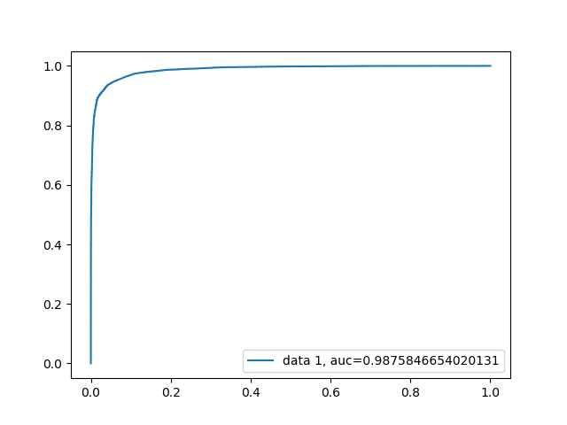
Logistics Regression ROC
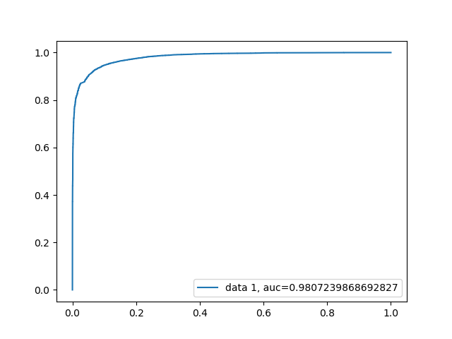
Linear Support Vector Machine ROC
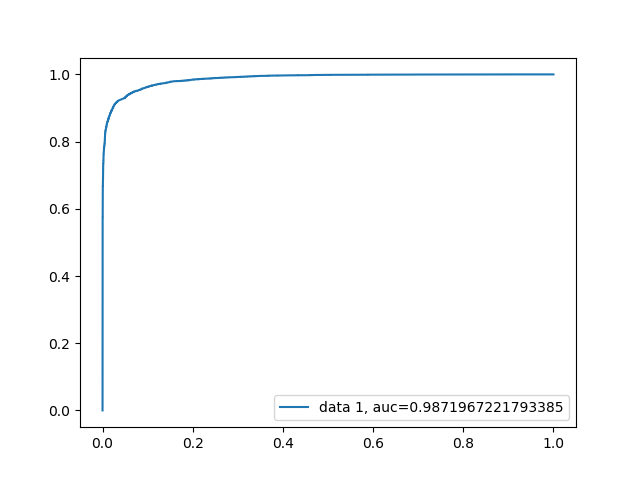
Naïve Bayes ROC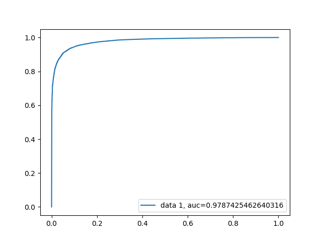
Random Forest Classifier ROC
By doing so we can see that while this model was able to classify a single tweet based on its content with a 94.98% success rate, this may not be the best way to flag trolls. Since a troll tweet will usually be output by the account multiple times, we can now look at our second hypothesis. Since we saw such an increase in success by removing the tweets that do not match with our calculated polarity, we will still apply the same filtering again. This time the dataset was slightly modified to be using 13 files instead of the original 1 from the malicious dataset since we need more accounts in the data vs just raw tweets. The number of clean tweets however was again kept at 50 thousand since that data we must force to be on the same account anyways. Every 100 tweets were linked as if it was coming from the same account. The classifiers were again kept at the same as the last two attempts and saw the following success rates:
| Classifier | Accuracy |
| Naïve Bayes | 97.91 |
| Logistic Regression | 100% |
| Linear Support Vector Machine | 100% |
| Random Forest Classifier | 100% |
| Averaging Ensemble (NB, LR, RFC) | 100% |
| Weighted Averaging Ensemble (NB, LR, RFC) | 100% |
ROC and AUC was calculated as such:
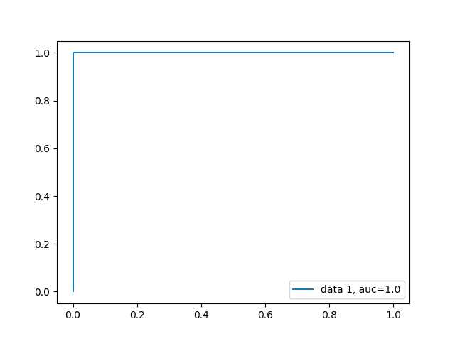
Naïve Bayes ROC
Linear Support Vector Machine ROC
Logistic Regression ROC
Probably the biggest problem with this hypothesis is that we are now overfitting based on our dataset. The overfitting is happening because the account-based approach now is causing the amount of malicious data and clean data to be significantly lower. With this approach the number of accounts is getting reduced to 3472 accounts in total and only 748 troll accounts and 2724 casual accounts. Even processing that much data took my computer almost 24 hours, so adding more accounts would lead to astronomical data processing times. While this is somewhat useful, it would probably be a better idea to take our individual tweet classifier approach and then look at each tweet in the account with it and classify the account based on how many tweets we said were malicious.
Model Execution TimeModel execution time in this case was kept minimal. The piece with this dataset that was the real killer in performance comes down to the data pre-processing, over 24 hours for the account-based approach. To get around this HDF format was used to dump the processed dataset to a file so that this would only have to be done once. After that the model training times were calculated as:
Hypothesis 1: (tweet categorizing)
| Classifier | Time |
| Naïve Bayes | 0.377 seconds |
| Logistic Regression | 1.552 seconds |
| Linear Support Vector Machine | 1.404 seconds |
| Random Forest Classifier | 1322.269 seconds |
| Averaging Ensemble | 194.902 seconds |
| Weighted Averaging Ensemble (NB, LR, RFC) | 194.453 seconds |
Hypothesis 2: (Account categorizing)
| Classifier | Time |
| Naïve Bayes | 0.010 seconds |
| Logistic Regression | 0.040 seconds |
| Linear Support Vector Machine | 0.025 seconds |
| Random Forest Classifier | 1.469 seconds |
| Averaging Ensemble | 3.045 seconds |
| Weighted Averaging Ensemble (NB, LR, RFC) | 1.855 seconds |
There was not much other work here to compare against. While our results perform well, we can compare against other sentiment analysis categorizing. Most of the other work on this dataset looked at using some of the other features provided in that dataset, thigs like tweet counts, date generated and the most used hashtags. This seems to be mildly successful and since the trolls generally contained defining characteristics like putting out a lot of tweets or using the same hashtags it is possible to classify them [3]. Part of the reason this analysis was not possible here is because gathering the “clean” dataset requires web scraping and was out of the scope for our approach. However, we can see that the bot that they trained in the article achieved a 97.9% AUC, which in our case is comparable. The dataset used in this article however is slightly different than ours and utilized actual journalists for the clean data, which would probably provide a good base point to perform this type of analysis on again if that data was readily available.
SummaryThe analysis done on the troll twitter dataset involved using Naïve Bayes, Logistic Regression, Linear Support Vector Machine, Random Forest Classifier, Averaging Ensemble, and Weighted Averaging Ensembling. With all of those we were able to successfully answer our original hypothesis as well as our newly added hypothesis. While classifying on an individual tweet might be useful the practicality of being able to flag an induvial tweet could land a lot of false positives. This idea lead to the second hypothesis which was found to be more accurate. Doing so requires a larger dataset to train and test off of but since both our datasets contained well over a million tweets that was a possibility. Python was used to perform all the analysis using Vader, SKLearn, NTLK, numpy, wordcloud, and matplotlib. The code is attached to the submission and each hypothesis attempt has its own python script, analysis_pandas.py for the first hypothesis and analysis_pandas_accounts.py for the second hypothesis. While answering both hypotheses are good approaches to this troll problem there still lies many possibilities for future growth. The “clean” data had to be manipulated to fit our attempt to classify on account basis, so a real dataset with actual account data would be more useful. Also using journalist accounts for the clean data would be a beneficial approach since the trolls in this dataset are all attempting to portray a journalist itself. We also restricted the dataset to only look at the Right and Left trolls which are not the only kind of trolls that were portrayed in this data. Adding those other types of accounts would help us further be able to classify the accounts but would also mean more data cleaning and analysis since the trends in some of those other accounts are hashtag based or in a language other than English.
While the account-based approach only resulted in overfitting on the dataset the tweet-based approach with cleaning out the non-matching polarity seemed to give the model the best success rate. We can use that model to classify tweets from an account and then approach with n out of m approach and say an account is a troll if 75% of the tweets from its account are flagged by our model. The account based approach could be looked at again however because I think it has a lot of potential but the amount of data needed to train the model needs to be processed in a better format and would need a fairly long time to even get the data into the correct format.
Resources[1] Boatwright, B. C.; Linvill, D. L.; and Warren, P. L. 2018. Troll factories: The internet research agency and state-sponsored agenda building. Resource Centre on Media Freedom in Europe.
[2] Starbird, K. (2018, October 17). A First Glimpse through the Data Window onto the Internet Research Agency's Twitter Operations. Retrieved April 30, 2019, from https://medium.com/@katestarbird/a-first-glimpse-through-the-data-window-onto-the-internet-research-agencys-twitter-operations-d4f0eea3f566
[3] Im, J; Chandrasekharan E; Sargent J; Lighthammer P; Denby T; Bhargava A; Hemphill L; Jurges D; Gilbert E; (2019, Jan 31). Still Out There: Modeling and Identifying Russian Troll Accounts on Twitter. University of Michigan and Georgia Institute of Technology


