Now that you have completed the first six assignments, it is time to complete your research project for the course. Include the following sections in your submission. Title Page Table of Contents Ex
SUN COAST STATISTICAL DATA ANALYSIS 0
Sun Coast Statistical Data Analysis
Jermaine Griffin
Data Analysis: Descriptive Statistics and Assumption Testing
Correlation: Descriptive Statistics and Assumption Testing
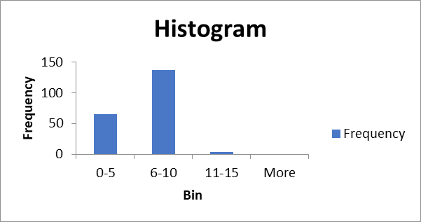
Frequency distribution table.
| Bin | Frequency |
| 0-5 | 65 |
| 6-10 | 137 |
| 11-15 | |
| More |
Histogram.
Descriptive statistics table.
| microns |
| mean annual sick days per employee |
|
| Mean | 5.657281553 | Mean | 7.126213592 |
| Standard Error | 0.255600143 | Standard Error | 0.186483898 |
| Median | Median | ||
| Mode | Mode | ||
| Standard Deviation | 2.59405814 | Standard Deviation | 1.892604864 |
| Sample Variance | 6.729137636 | Sample Variance | 3.58195317 |
| Kurtosis | -0.852161902 | Kurtosis | 0.124922603 |
| Skewness | -0.373257127 | Skewness | 0.142249784 |
| Range | 9.8 | Range | 10 |
| Minimum | 0.2 | Minimum | |
| Maximum | 10 | Maximum | 12 |
| Sum | 582.7 | Sum | 734 |
| Count | 103 | Count | 103 |
| Largest(1) | 10 | Largest(1) | 12 |
| Smallest(1) | 0.2 | Smallest(1) |
Measurement scale.
Ratio scale was used since it has all of the features of interval scale and a true zero, which refers to complete absence of the characteristic being measured. This scale was used because microns refers to length which can be effectively described using ratio scale. Also, the mean annual sick days per employee is a number that is well described using the ratio scale (Peacock, 2019).
Measure of central tendency.
From the above descriptive statistics table, the mean, mode, and median for mean annual sick days per employee are;
Mean: 7.126213592
Medium: 7
Mode: 7
Also for the Microns, the mean, mode, and medium are;
Mean: 5.657281553
Medium: 6
Mode: 8
Evaluation.
From the descriptive statistics, for microns, the skewness was -0.373257127 while the kurtosis was -0.852161902, on the other hand, for mean annual sick days per employee, skewness was 0.142249784 and kurtosis was 0.124922603, it must be noted that for normality test assumption, the skewness must be within a +-2 range while kurtosis between +-7 range. However according to the descriptive statistical values above, the skewness and kurtosis ranges aren’t within the intended range for normality assumption qualification. Therefore the parametric statistical testing were not met.
Simple Regression: Descriptive Statistics and Assumption Testing
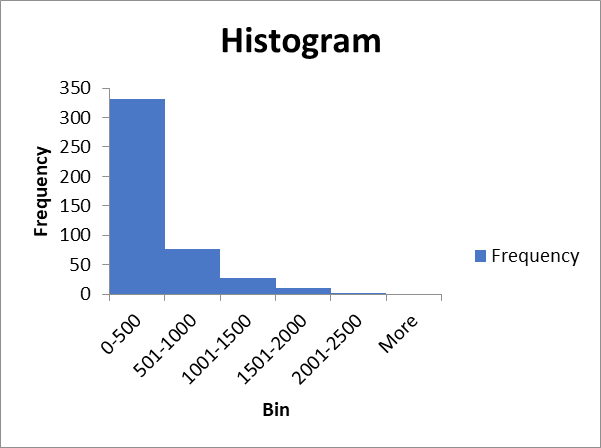
Frequency distribution table.
| Bin | Frequency |
| 0-500 | 331 |
| 501-1000 | 76 |
| 1001-1500 | 27 |
| 1501-2000 | 11 |
| 2001-2500 | |
| More |
Histogram.
Descriptive statistics table.
| safety training expenditure |
| lost time hours |
|
| Mean | 595.9843812 | Mean | 188.0044843 |
| Standard Error | 31.4770075 | Standard Error | 4.803089447 |
| Median | 507.772 | Median | 190 |
| Mode | 234 | Mode | 190 |
| Standard Deviation | 470.0519613 | Standard Deviation | 71.72542099 |
| Sample Variance | 220948.8463 | Sample Variance | 5144.536016 |
| Kurtosis | 0.444080195 | Kurtosis | -0.501223533 |
| Skewness | 0.951331922 | Skewness | -0.081984874 |
| Range | 2251.404 | Range | 350 |
| Minimum | 20.456 | Minimum | 10 |
| Maximum | 2271.86 | Maximum | 360 |
| Sum | 132904.517 | Sum | 41925 |
| Count | 223 | Count | 223 |
| Largest(1) | 2271.86 | Largest(1) | 360 |
| Smallest(1) | 20.456 | Smallest(1) | 10 |
Measurement scale.
Ratio scale was used since it has all of the features of interval scale and a true zero, which refers to complete absence of the characteristic being measured. This scale was used because safety training expenditure refers to length which can be effectively described using ratio scale. Also, the lost time hours are numbers that are well described using the ratio scale (McCarthy, R. McCarthy, M, Ceccucci, & Halawi, 2019).
Measure of central tendency.
From the above descriptive statistics table, the mean, mode, and median for safety training expenditure are;
Mean: 595.9843812
Medium: 507.772
Mode: 234
For the lost time hours, the mean, mode, and medium are;
Mean: 188.0044843
Medium: 190
Mode: 190
Evaluation.
From the descriptive statistics, for safety training expenditure, the skewness was -0.951331922 while the kurtosis was 0.444080195, on the other hand, for lost time hours, skewness was -0.081984874 and kurtosis was -0.501223533, it must be noted that for normality test assumption, the skewness must be within a +-2 range while kurtosis between +-7 range. However according to the descriptive statistical values above, the skewness and kurtosis ranges aren’t within the intended range for normality assumption qualification. Therefore the parametric statistical testing were not met (Ma’arif, Motahar, & Mohd Satar, 2018).
Multiple Regression: Descriptive Statistics and Assumption Testing
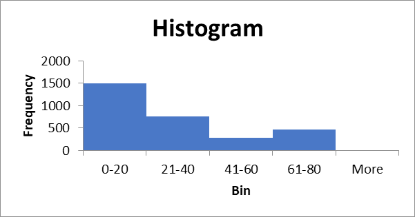
Frequency distribution table.
| Bin | Frequency |
| 0-20 | 1503 |
| 21-40 | 761 |
| 41-60 | 277 |
| 61-80 | 465 |
| More |
Histogram.
Descriptive statistics table.
| Chord Length |
| Velocity |
|
| Mean | 0.116140053 | Mean | 50.86074518 |
| Standard Error | 0.001256368 | Standard Error | 0.401686079 |
| Median | 0.1176 | Median | 39.6 |
| Mode | 0.0917 | Mode | 39.6 |
| Standard Deviation | 0.048707555 | Standard Deviation | 15.5727844 |
| Sample Variance | 0.002372426 | Sample Variance | 242.5116138 |
| Kurtosis | -1.178196484 | Kurtosis | -1.563951274 |
| Skewness | -0.027537436 | Skewness | 0.235852414 |
| Range | 0.1697 | Range | 39.6 |
| Minimum | 0.03 | Minimum | 31.7 |
| Maximum | 0.1997 | Maximum | 71.3 |
| Sum | 174.5585 | Sum | 76443.7 |
| Count | 1503 | Count | 1503 |
| Largest(1) | 0.1997 | Largest(1) | 71.3 |
| Smallest(1) | 0.03 | Smallest(1) | 31.7 |
Measure of central tendency.
From the above descriptive statistics table, the mean, mode, and median for Chord Length are;
Mean: 0.116140053
Medium: 0.1176
Mode: 0.0917
For the Velocity, the mean, mode, and medium are;
Mean: 50.86074518
Medium: 39.6
Mode: 39.6
Evaluation.
From the descriptive statistics, for Chord Length, the skewness was -0.027537436 while the kurtosis was -1.178196484, on the other hand, for Velocity, skewness was 0.235852414 and kurtosis was -1.563951274, it must be noted that for normality test assumption, the skewness must be within a +-2 range while kurtosis between +-7 range (Qiu, Wei, & Bai, 2017). However according to the descriptive statistical values above, the skewness and kurtosis ranges aren’t within the intended range for normality assumption qualification. Therefore the parametric statistical testing were not met.
Independent Samples t Test: Descriptive Statistics and Assumption Testing
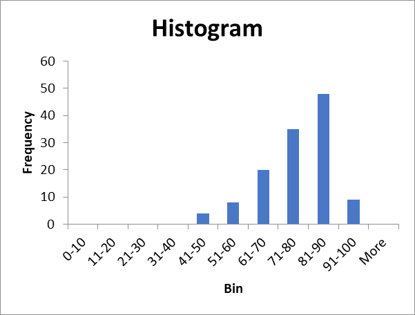
Frequency distribution table.
| Bin | Frequency |
| 0-10 | |
| 11-20 | |
| 21-30 | |
| 31-40 | |
| 41-50 | |
| 51-60 | |
| 61-70 | 20 |
| 71-80 | 35 |
| 81-90 | 48 |
| 91-100 | |
| More |
Histogram.
Descriptive statistics table.
| Group A Prior Training Scores |
| Group B Revised Training Scores |
|
| Mean | 69.79032258 | Mean | 84.77419355 |
| Standard Error | 1.402788093 | Standard Error | 0.659478888 |
| Median | 70 | Median | 85 |
| Mode | 80 | Mode | 85 |
| Standard Deviation | 11.04556449 | Standard Deviation | 5.192741955 |
| Sample Variance | 122.004495 | Sample Variance | 26.96456901 |
| Kurtosis | -0.77667598 | Kurtosis | -0.352537913 |
| Skewness | -0.086798138 | Skewness | 0.144084526 |
| Range | 41 | Range | 22 |
| Minimum | 50 | Minimum | 75 |
| Maximum | 91 | Maximum | 97 |
| Sum | 4327 | Sum | 5256 |
| Count | 62 | Count | 62 |
| Largest(1) | 91 | Largest(1) | 97 |
| Smallest(1) | 50 | Smallest(1) | 75 |
Measurement scale.
Ratio scale was used since it has all of the features of interval scale and a true zero, which refers to complete absence of the characteristic being measured. This scale was used because Group A Prior Training Scores can be treated as student marks which can be treated as measurement values which can be effectively described using ratio scale. Also, the Group B Revised Training Scores can as well as classified as values that are well described using the ratio scale (Stypulkowski, Bernardeau, & Jakubowski, 2018).
Measure of central tendency.
From the above descriptive statistics table, the mean, mode, and median for Group A Prior Training Scores are;
Mean: 69.79032258
Medium: 70
Mode: 80
For the Group B Revised Training Scores, the mean, mode, and medium are;
Mean: 84.77419355
Medium: 85
Mode: 85
Evaluation.
From the descriptive statistics, for Group A Prior Training Scores, the skewness was --0.086798138 while the kurtosis was -0.77667598, on the other hand, for Group B Revised Training Scores, skewness was 0.144084526 and kurtosis was -0.352537913, it must be noted that for normality test assumption, the skewness must be within a +-2 range while kurtosis between +-7 range. However according to the descriptive statistical values above, the skewness and kurtosis ranges aren’t within the intended range for normality assumption qualification. Therefore the parametric statistical testing were not met (Wang, et al. 2019).
Dependent Samples (Paired-Samples) t Test: Descriptive Statistics and Assumption Testing
Frequency distribution table.
| Bin | Frequency |
| 0-10 | |
| 11-20 | 12 |
| 21-30 | 18 |
| 31-40 | 28 |
| 41-50 | 32 |
| 51-60 | |
| More |
Histogram.

Descriptive statistics table.
| Pre-Exposure μg/dL |
| Post-Exposure μg/dL |
|
| Mean | 32.85714286 | Mean | 33.28571429 |
| Standard Error | 1.752306546 | Standard Error | 1.781423416 |
| Median | 35 | Median | 36 |
| Mode | 36 | Mode | 38 |
| Standard Deviation | 12.26614582 | Standard Deviation | 12.46996391 |
| Sample Variance | 150.4583333 | Sample Variance | 155.5 |
| Kurtosis | -0.576037127 | Kurtosis | -0.654212507 |
| Skewness | -0.425109654 | Skewness | -0.483629097 |
| Range | 50 | Range | 50 |
| Minimum | Minimum | ||
| Maximum | 56 | Maximum | 56 |
| Sum | 1610 | Sum | 1631 |
| Count | 49 | Count | 49 |
| Largest(1) | 56 | Largest(1) | 56 |
| Smallest(1) | Smallest(1) |
Measurement scale.
Ratio scale was used since it has all of the features of interval scale and a true zero, which refers to complete absence of the characteristic being measured. This scale was used because Pre-Exposure μg/dL parameters can be treated as measurement values which can be effectively described using ratio scale. Also, the Pre-Exposure μg/dL refers to measurement values that are well described using the ratio scale (Berghoff, et al. 2016).
Measure of central tendency.
From the above descriptive statistics table, the mean, mode, and median for Pre-Exposure μg/dL are;
Mean: 32.85714286
Medium: 35
Mode: 36
For the Post-Exposure μg/dL, the mean, mode, and medium are;
Mean: 33.28571429
Medium: 36
Mode: 38
Evaluation.
From the descriptive statistics, for Pre-Exposure μg/dL, the skewness was -0.425109654 while the kurtosis was -0.576037127, on the other hand, for Post-Exposure μg/dL, skewness was -0.483629097 and kurtosis was -0.654212507, it must be noted that for normality test assumption, the skewness must be within a +-2 range while kurtosis between +-7 range. However according to the descriptive statistical values above, the skewness and kurtosis ranges aren’t within the intended range for normality assumption qualification. Therefore the parametric statistical testing were not met (Barkana, Saricicek, & Yildirim, 2017).
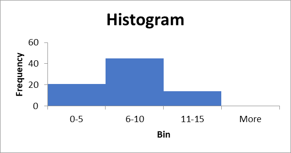
ANOVA: Descriptive Statistics and Assumption Testing
Frequency distribution table.
| Bin | Frequency |
| 0-5 | 21 |
| 6-10 | 45 |
| 11-15 | 14 |
| More |
Histogram.
Descriptive statistics table.
| A = Air |
| B = Soil |
| C = Water |
| D = Training |
|
| Mean | 8.9 | Mean | 9.1 | Mean | Mean | 5.4 | |
| Standard Error | 0.68 | Standard Error | 0.39 | Standard Error | 0.58 | Standard Error | 0.3 |
| Median | Median | Median | Median | ||||
| Mode | 11 | Mode | Mode | Mode | |||
| Standard Deviation | 3.06 | Standard Deviation | 1.74 | Standard Deviation | 2.58 | Standard Deviation | 1.2 |
| Sample Variance | 9.36 | Sample Variance | 3.04 | Sample Variance | 6.63 | Sample Variance | 1.4 |
| Kurtosis | -0.6 | Kurtosis | 0.12 | Kurtosis | -0.2 | Kurtosis | 0.3 |
| Skewness | -0.4 | Skewness | 0.49 | Skewness | 0.76 | Skewness | 0.2 |
| Range | 11 | Range | Range | Range | |||
| Minimum | Minimum | Minimum | Minimum | ||||
| Maximum | 14 | Maximum | 13 | Maximum | 12 | Maximum | |
| Sum | 178 | Sum | 182 | Sum | 140 | Sum | 108 |
| Count | 20 | Count | 20 | Count | 20 | Count | 20 |
| Largest(1) | 14 | Largest(1) | 13 | Largest(1) | 12 | Largest(1) | |
| Smallest(1) | Smallest(1) | Smallest(1) | Smallest(1) |
Measurement scale.
In this statistical descriptive analysis, the nominal scale have been used. In this case, the letters that is A, B, C and D have been used to identify or denote items. For instance, A has been used to denote Air, B has been used to denote Soil, and C have been used to denote Water and finally, D have been used to denote Training. However, it should be noted that the letters aren’t used to denote the specialty of an item in relation to another, they are just applied for identity (Innocenti, et al. 2017).
Measure of central tendency.
From the above descriptive statistics table, the mean, mode, and median for air are;
Mean: 8.9
Medium: 9
Mode: 11
Also for the soil, the mean, mode, and medium are;
Mean: 9.1
Medium: 9
Mode: 8
For water, the mean, mode, and medium are;
Mean: 7
Medium: 6
Mode: 6
For the training, the mean, mode, and medium are;
Mean: 5.4
Medium: 5
Mode: 5
Evaluation.
From the descriptive statistics, for Air, the skewness was -0.4 while the kurtosis was -0.6, on the other hand, for Soil, skewness was 0.49 and kurtosis was 0.12, also for Water, the skewness was 0.76 while the kurtosis was -0.2, on the other hand, for Training, skewness was 0.2 and kurtosis was 0.3 it must be noted that for normality test assumption, the skewness must be within a +-2 range while kurtosis between +-7 range. However according to the descriptive statistical values above, the skewness and kurtosis ranges aren’t within the intended range for normality assumption qualification. Therefore the parametric statistical testing were not met (Peacock, 2019).
References
Barkana, B. D., Saricicek, I., & Yildirim, B. (2017). Performance analysis of descriptive statistical features in retinal vessel segmentation via fuzzy logic, ANN, SVM, and classifier fusion. Knowledge-Based Systems, 118, 165-176.
Berghoff, A. S., Schur, S., Füreder, L. M., Gatterbauer, B., Dieckmann, K., Widhalm, G., ... & Preusser, M. (2016). Descriptive statistical analysis of a real life cohort of 2419 patients with brain metastases of solid cancers. ESMO open, 1(2), e000024.
Innocenti, A., Mori, F., Melita, D., Dreassi, E., Ciancio, F., & Innocenti, M. (2017). Evaluation of long-term outcomes of correction of severe blepharoptosis with advancement of external levator muscle complex: descriptive statistical analysis of the results. in vivo, 31(1), 111-115.
Ma’arif, M. Y., Motahar, S. M., & Mohd Satar, N. S. (2018). A descriptive statistical based analysis on perceptual of ERP training needs. In Proceedings of 2018 International Conference on Engineering, Science, and Application (ICESA 2018) (pp. 46-62).
McCarthy, R. V., McCarthy, M. M., Ceccucci, W., & Halawi, L. (2019). What Do Descriptive Statistics Tell Us. In Applying Predictive Analytics (pp. 57-87). Springer, Cham.
Peacock, H. (2019). Descriptive Statistical Analysis using SPSS.
Qiu, Y., Wei, M., & Bai, B. (2017). Descriptive statistical analysis for the PPG field applications in China: Screening guidelines, design considerations, and performances. Journal of Petroleum Science and Engineering, 153, 1-11.
Stypulkowski, J. B., Bernardeau, F. G., & Jakubowski, J. (2018). Descriptive statistical analysis of TBM performance at Abu Hamour Tunnel Phase I. Arabian Journal of Geosciences, 11(9), 191.
Wang, Y., Shao, X., Liu, C., Cai, G., Kou, L., & Wu, Z. (2019). Analysis of wind farm output characteristics based on descriptive statistical analysis and envelope domain. Energy, 170, 580-591.


