Microeconomics questions and answers explained, please.
CHAPTER 9: Profit Maximization in Perfectly Competitive Markets
CHAPTER 9
Profit Maximization in Perfectly Competitive Markets
CHAPTER ANALYSISTo maximize profits, firms must consider both cost and demand conditions. This chapter explores the firm’s demand curve. The demand curve shows sales revenue at various volumes of output. The model of perfect competition is presented, and a discussion of how firms respond to changes in price and cost in a perfect market is provided. In addition, the discussion is extended to include both long run and short run responses by the firm.
9.1 The Assumption of Perfect Competition
Perfect competition refers to an economic state characterized by four assumptions:
1. There are a large number of buyers and sellers such that all participants in the market are price takers. Section 9.3 in the text justifies and explains this assumption.
2. There is unrestricted mobility of resources, or free entry and exit. This assumption is necessary in order to reach long-run equilibrium. Section 9.7 in the text provides a more detailed discussion of this assumption.
3. It is assumed that the firms produce a homogeneous product implying that the goods are perfect substitutes.
4. It is assumed that firms and consumers possess all relevant information necessary to make economic decisions.
9.2 Profit Maximization
We also assume profit maximization is the primary goal of the firm. While this assumption is often controversial, it is still used because it has proven to predict well. The survivor principle suggests that in competitive markets, firms will only survive if they engage in profit maximizing behavior. Firms that do not engage in such behavior will fail. This principle supports the profit maximization assumption.
9.3 The Demand Curve Facing the Competitive Firm
A perfectly competitive firm faces a horizontal demand curve, which means that the firm can sell as much as it can produce at the market price. The competitive firm is a price taker which implies it must accept the price determined in the marketplace. For example, laborers looking for jobs are not able to set their wages. Rather, the market determines their wages. If an individual will not work for the market wage, someone else will. Similarly, wheat farmers cannot get more than the market price for their wheat because the amount they supply individually is so small relative to the entire market. The horizontal demand curve has an elasticity of infinity, which implies if one firm was to increase its price, quantity demand will decrease by infinite amounts. Since the product sold is homogeneous, consumers would just buy the product from one of the many other firms that exist.
In addition, the demand curve is also the firm's average revenue curve and its marginal revenue curve. Average revenue is equal to total revenue divided by output. Marginal revenue is equal to the change in total revenue divided by the change in output. Section 9.3 in the text provides a more detailed explanation of these concepts.
9.4 Short-Run Profit Maximization
In the short run, the firm faces two decisions: 1) How much q to produce in order to maximize profit and 2) given its profit, should the firm stay open or shut down. In order to maximize profit the firm must choose that level of output (q) where marginal revenue (MR) is equal (or the closest in value) to marginal cost (MC). Total profit is equal to total revenue (TR) minus total cost (TC). Therefore, in order to maximize profit, the firm wants to choose output where the distance between total revenue and total costs is the greatest. Figure 9.2 in the text provides a graphical depiction of this concept.
Table 9.1 in the text provides a numerical example of a perfectly competitive firm in the short run. The firm needs to choose that level of q where it will maximize its profits. Since firms make decisions at the margin, it will look at each potential level of output it can produce and decide whether producing that given output is profitable. For example, at q = 2, marginal revenue exceeds marginal cost implying it is profitable to produce 2 units. Next, the firm needs to determine if producing 3 units is profitable. Again, marginal revenue exceeds marginal cost so the firm will produce 3 units. Therefore, when marginal revenue exceeds marginal cost, the firm can increase its profits by producing that unit. The firm will keep doing this until marginal revenue is equal to marginal cost. At higher levels of output, for example q = 10, marginal costs exceeds marginal revenue so the firm will not produce the 10th unit. Marginal revenue is closest to marginal costs when q = 8. At this point we also see profit is equal to $11.10 which is the highest value in the profit column. Take note that there is a difference between total profit, which is equal to total revenue minus total cost, and average profit which is equal to total profit divided by output.
Figure 9.3 in the text illustrates the short run situation of the perfectly competitive firm. In order to graphically show the firm’s level of profit, we need to look at the relationship between the firm’s price and its average total and average variable cost curves at the profit maximizing level of q. If the price is greater than average total cost, the firm is making positive profit. If price is equal to average total cost, the firm’s profit is equal to zero which implies the firm is breaking even. If price fall in between average total cost and average variable cost, the firm is making negative profit but the firm would still stay open. Since the firm always has to pay its fixed cost, the firm would incur a greater negative profit by shutting down. This situation is depicted in Figure 9.4. However, if the price is equal to or less than average variable cost, the firm should shut down. In Figure 9.3, the firm’s price is greater than average total cost which means it is making positive profit and should therefore stay open.
9.5 The Perfectly Competitive Firm’s Short-Run Supply Curve
In the short run, the perfectly competitive firm’s short run supply curve is equal to the portion of its marginal cost curve that lies above the minimum point of the firm’s average variable cost curve. The minimum point on a firm’s average variable cost curve is referred to as the shutdown point. Therefore, the firm’s supply curve shows the relationship between price and profitable output levels. The portion of the marginal cost curve that lies below the minimum average variable cost is not relevant since the firm does not produce any output at those price levels.
The firm’s short run supply curve is affected by a change in input prices. Since a change in an input price implies a change in costs, it will cause the marginal cost curve to shift. Suppose there is a decrease in costs. This will shift the marginal cost curve to the right. Figure 9.6 in the text shows the increase in output that occurs due to these lower costs.
9.6 The Short Run Industry Supply Curve
The industry short-run supply curve is found by horizontally summing the supply curves of the firms in the industry. Figure 9.7 of the text shows the derivation of the industry supply curve. Note, too, that the derivation assumes input prices are fixed because the marginal cost of the firm shifts when input prices change. Since the marginal cost curves are upward sloping, the industry supply curve is upward sloping as well. . The competitive model is completed by adding the industry demand. The intersection of the industry demand curve and supply curve determines the market price and the market level of output.
9.7 Long-Run Competitive Equilibrium
Based on profitability in the short run, the firm needs to decide whether it should exit or remain in the industry. It is important to understand the difference between shut down and exit. When the firm shuts down, it implies output is equal to zero, but the firm still has to pay its fixed cost because capital in the short run is fixed. In the long run, both capital and labor can change. Therefore, the firm is able to eliminate its fixed cost because the firm can sell off its capital. Once the firm has done away with both labor and capital, it implies it has exited the industry.
In the long run, a perfectly competitive firm’s profit will always equal zero. Zero economic profit is the point where the price is equal to the average cost of production. Suppose the firm is making positive profit in the short run. The firm will remain in the industry, but now potential firms will enter because they want to earn the positive profits as well. As more firms enter, the industry supply curve will shift to the right driving down the price, and therefore decreasing profit. Firms will continue to enter until price eventually falls enough to equal minimum average total cost. At this point, the firm is making zero profit and is breaking even. When zero profits exist, outside firms have no incentive to enter. This concept is depicted by Figure 9.9 in the text.
Now suppose some firms were making negative profit in the short run. In the long run these firms will exit the industry. As firms exit, the industry supply curve will shift to the left leading to an increase in price. As price goes up, profits become less negative. This will continue until the price increases to equal minimum average total cost. Once this occurs, profits are zero and there is no incentive for exit or entry. Therefore, the long run equilibrium for a perfectly competitive industry is characterized by zero profit.
9.8 The Long-Run Industry Supply Curve
The long-run supply curve shows the relationship between price and industry output. The slope of the long run supply curve depends on what happens to input prices as the industry expands or contracts. A constant cost industry is one in which the expansion of output does not increase input prices. If this is the case, it means long run average costs are constant and the industry supply curve is horizontal. An increasing cost industry is when expansion of output leads to an increase in input prices. This implies higher long run average costs and therefore an upward sloping long run supply curve. Finally, a decreasing cost industry is one where an expansion of output leads to a decrease in input prices. This leads to a decrease in long run average cost and a long run supply curve that is downward sloping. Note that a downward sloping industry supply curve is a rare and highly unusual case.
9.9 When Does the Competitive Model Apply?
While is important to know how the competitive model works, it is also essential to be able to use it to analyze real-world phenomena. Of the four assumptions listed in Section 9.1, two of these are vital to the workings of the model. The first is that there are a large amount of firms implying they are price takers. The second is the assumption of free entry and exit which generates the zero profit long run equilibrium condition. When there are restrictions on entry and exit, the competitive adjustment process cannot work properly, and long-run profits can be made by firms in the industry.
In reality, all four assumptions are rarely satisfied in real world markets. The industry that comes closest to qualifying as perfectly competitive is agricultural goods. For example, consider the market for corn. There are a large number of farms that produce corn, corn is almost homogeneous, there are little if any restrictions on entry and exit, and information on corn is readily available.
9.10 The Mathematics Behind Perfect Competition (online only content)
Total profit for a firm is the difference between total revenue and total cost:
π = R – C.
Total revenue is equal to price times output (P)(Q). Since price is a constant for a competitive firm (P0), the total profit for a firm is:
π = P0Q – C.
Since the first order condition for finding the profit maximizing output requires that the first derivative of the total profit function equal to zero, we get:
dπ/dQ = P0 (dQ/dQ) – (dC/dQ) = 0;
= P0 - MC = 0.
So, we know that the competitive firm should produce an output where MC = P0
Looking at the second order condition for profit maximization:
d2π/dQ2 = 0 - d2C/dQ2 < 0.
We know that for profit to be at a maximum, d2C/dQ2 must be positive. So, when price equals marginal cost, the marginal cost curve must have a positive slope.
ILLUSTRATIONS
Going Out of BusinessA firm will shut down in the short run when price is below average variable cost, and it will go out of business in the long run when price is below long run average cost at every level of output. Evidence of this behavior can be seen in virtually any town in the country. For example, a building that once was a gas station is now an auto repair shop or a convenience store. A building that at one time housed a laundry mat now houses a pizza parlor; a tanning spa becomes a clothing store. In each case, a former business shut down because its price was too low to cover its variable costs, and eventually it went out of business. The durable assets are then transferred to another industry.
The Historical Development of Perfect Competition
The model of perfect competition described in the textbook evolved over time. Adam Smith discussed competition, but used the term more as popular discussion. That is, it denoted the idea of rivalry. George Stigler traced out the development of the concept of "perfect competition". He identified five conditions of competition that Smith noted: (1) the rivals must act independently; (2) the number of rivals must be enough to eliminate extraordinary gains; (3) the agents must have, "...tolerable knowledge of the market opportunities"; (4) there must be freedom to act on the knowledge, i.e., there must not be social barriers to entry or exit; and (5) enough time for resources to flow in the more profitable directions must elapse.
Stigler then traced out the manner in which economists altered and refined these points over time. Finally, in the early part of the last century, the assumptions used in the text were articulated. The result has been that the model of perfect competition is not a model of how firms behave or a model of competition as a process. In other words, there is no competitive behavior in the model of perfect competition. Instead, the model allows us to analyze how markets operate. As such, the model has proven to be very useful.
[For details see George J. Stigler, "Perfect Competition, Historically Contemplated," In The Essence of Stigler, ed. by Kurt R. Leube and Thomas Gale Moore (Stanford: Hoover Institution Press, 1986), pp. 265-88).]
KEY CONCEPTS
perfect competition average profit per unit
free entry and exit short-run firm supply curve
homogeneous product shutdown point
survivor principle short-run industry supply curve
price taker zero economic profit
average revenue long-run industry supply curve
marginal revenue constant-cost industry
total revenue increasing-cost industry
total profit decreasing-cost industry
profit maximization
REVIEW QUESTIONS
True/False1. In the model of perfect competition, consumers are assumed to view the products of the various firms in the industry as perfect substitutes.
2. If it can be shown that some firms do not seek to maximize profits, then the assumption of profit maximization is invalid.
3. A perfectly competitive firm is a price taker because the firm must take the market price as given.
4. The demand curve for a perfectly competitive firm is also its marginal revenue curve.
5. If MC > MR, the firm should produce at a larger level of output.
6. If P < ATC, the firm will shut down to minimize its losses.
7. A perfectly competitive firm makes zero profits in long-run equilibrium.
8. When input prices are held constant, the short-run industry supply curve is derived by summing the firms' marginal cost curves horizontally.
9. The law of diminishing marginal returns is the basic determinant of the shape of the industry's short-run supply curve.
10. A perfectly competitive firm responds to a higher price by increasing its level of output.
11. In the short run, an increase in market demand leads to a larger level of output because new firms enter the industry.
12. A competitive industry's long-run supply curve is determined by how a change in industry output affects the prices of inputs.
13. The supply curves of inputs remain unchanged along an industry's long-run supply curve.
14. Economic profits are zero along a long-run supply curve.
15. The shape of the long-run supply curve depends on the supply curves of inputs.
Multiple Choice/Short Answer
1. If a firm is a price taker, then its demand curve is
a. downward sloping.
b. vertical.
c. horizontal
d. upward sloping.
2. Firms will consider themselves price takers when
a. there is unrestricted mobility of resources.
b. they collude with other firms.
c. they produce a heterogeneous product.
d. there are a large number of competing firms producing a homogeneous product.
3. For a competitive firm, the demand curve is also
a. a total revenue curve.
b. an average revenue curve.
c. a marginal revenue curve.
d. both b and c.
4. The price elasticity of demand for a perfectly competitive firm is
a. less than 1.
b. greater than 1 but less than infinite.
c. infinite.
d. uncertain without more information.
5. Profits are maximized where
a. TR = TC.
b. TR - TC = 0.
c. the slope of the total revenue curve exceeds the slope of the total cost curve by the largest margin.
d. total revenues exceed total cost by the largest amount possible.
6. Profits are maximized where
a. MR = MC.
b. P = ATC.
c. price exceeds marginal cost by the largest amount.
d. the slope of the marginal revenue curve equals the slope of the marginal cost curve.
Questions 7 to 11 refer to Figure 9-1.

7. If the price is P1, what is the profit-maximizing level of output?
8. If the price is P4, what is the profit-maximizing level of output?
9. If the price is P3, what is the value of the firm's profits?
10. What is the minimum level of output the firm will produce before shutting down?
11. What points are on the supply curve of the firm?
a. A, B, C, and D.
b. A, B, and C only.
c. C and D only.
d. B, C, and D only.
12. If MR > MC, output should
a. expand.
b. contract.
c. remain constant.
d. expand or contract depending on whether P > AC.
13. A perfectly competitive firm will shut down in the short run when
a. ATC > P > AVC.
b. AVC > P > ATC.
c. AVC > P.
d. ATC > P.
14. The short-run industry supply curve slopes upward because
a. the long-run supply curve slopes upward.
b. of the existence of fixed costs in the short run.
c. of the law of diminishing marginal returns.
d. of decreasing returns to scale.
15. In the short run, an increase in demand will
a. induce firms to charge a higher price and produce at the same level of output.
b. induce firms to produce at a larger level of output as price increases.
c. generate a low price as the quantity supplied increases.
d. induce higher wages for workers in the industry.
16. In long-run equilibrium a perfectly competitive firm earns
a. zero profits.
b. modest profits.
c. profits, but we cannot say how large the profits will be.
d. profits until new firms enter the industry.
17. For a competitive firm, as price increases
a. output decreases.
b. output stays the same, since the size of the plant is fixed in the short run.
c. output increases.
d. output will either increase or decrease depending on the shape of the firm's average cost curve.

18. Refer to Figure 9-2. If industry demand increases from D1 to D2, then
a. the firm's output will be q1 in the short run and q2 in the long run.
b. industry output increases from Q1 to Q2 as new firms enter the industry.
c. the firm can make a profit by changing a price below P2 and take business away from the other firms.
d. each firm increases output from q1 to q2 and earns economic profits in the short run.
19. If firms are making profits in the short run, then
a. new firms will enter the industry until profits are zero.
b. firms will make profits in the long run too.
c. firms must not be price takers.
d. cost curves are not defined properly.
20. The key to the long-run adjustment in a competitive industry is
a. the shape of the short-run supply curves.
b. the market price elasticity of demand.
c. profit seeking by firms.
the price-taking behavior of firms.
21. The shape of the industry long-run supply curve depends on
a. the shape of the firms' short-run supply curves.
b. the number of firms in the industry.
c. whether new firms enter the industry.
d. what happens to input prices as industry output expands.
22. Along an industry long-run supply curve
a. input prices are held constant.
b. the number of firms in the industry is constant.
c. economic profits increase at higher rates of output.
d. economic profits are zero.
23. What is the value of the long-run price elasticity of supply of a constant-cost industry?
a. 0
b. 1
c. Between -l and +1
d. Infinity
24. If the price of the variable input decreases, what happens to the rate of output of the firm?
a. Increases.
b. Decreases.
c. Remains constant.
d. Cannot tell without more information.
25. Which of the four assumptions of the competitive model is (are) necessary for the industry to reach the condition of long-run equilibrium? (There may be more than one answer.)
a. Large number of firms
b. Unrestricted resource mobility
c. Homogeneous product
d. All relevant information is known.
Discussion Questions and Problems
1. a. List the four assumptions of perfect competition and state the function of each assumption.
b. Are there any industries in which these assumptions are fairly realistic?
c. Can the perfect competition model be used in industries where the assumptions are not realistic?
2. Explain why a competitive firm's demand curve is also its marginal revenue curve and its average revenue curve.
3. Use the data in Discussion Question 1 of Chapter 8 in the Study Guide and apply it to a competitive firm.
a. If price is 90 cents, what rate of output will the firm produce? Why? Calculate the firm's profits.
b. If price is $1.67 what rate of output will the firm produce? Why? Calculate the firm's profits.
If price is $5.00, what rate of output will the firm produce? Why? Calculate the firm's profits.
d. What is the shutdown point of the firm?
e. Is there a relationship between price and output for the firm? If so, what is it?
4. State the short-run profit-maximizing rule for a firm and explain why it ensures that profits are maximized.
5. State the condition under which a competitive firm will go out of business and explain why it will do so.
6. Use the data in Discussion Question 1 of Chapter 8 in the Study Guide and let there be 100 firms in the industry. Find the points on the industry supply curve. If you graphed it, what would be its shape? Why?
7. Explain the following statement taken from the text: ". . . we do not need to use the average cost curves to explain the determination of price and quantity in the short run. All the necessary information is contained in the industry supply and demand curves".
8. Why will a firm continue to operate in the long run when it is earning zero profits?
9. What happens to the durable assets of a firm when it goes out of business?
10. Is it possible for fixed costs to increase in the short run? Explain.
11. Use the data in Discussion Questions 1 and 3 of Chapter 8 in the Study Guide.
a. If price is $2.50 and the price of fertilizer is $50 and land rents for $500, what is the profit-maximizing level of output? How many units of fertilizer does the firm use? Calculate the firm's profits.
b. Suppose the price of fertilizer falls to $25. What level of output will the firm produce? How many units of fertilizer will it buy now? Calculate the firm's profits.
c. Is the level of output found in part b a short-run equilibrium? Explain.
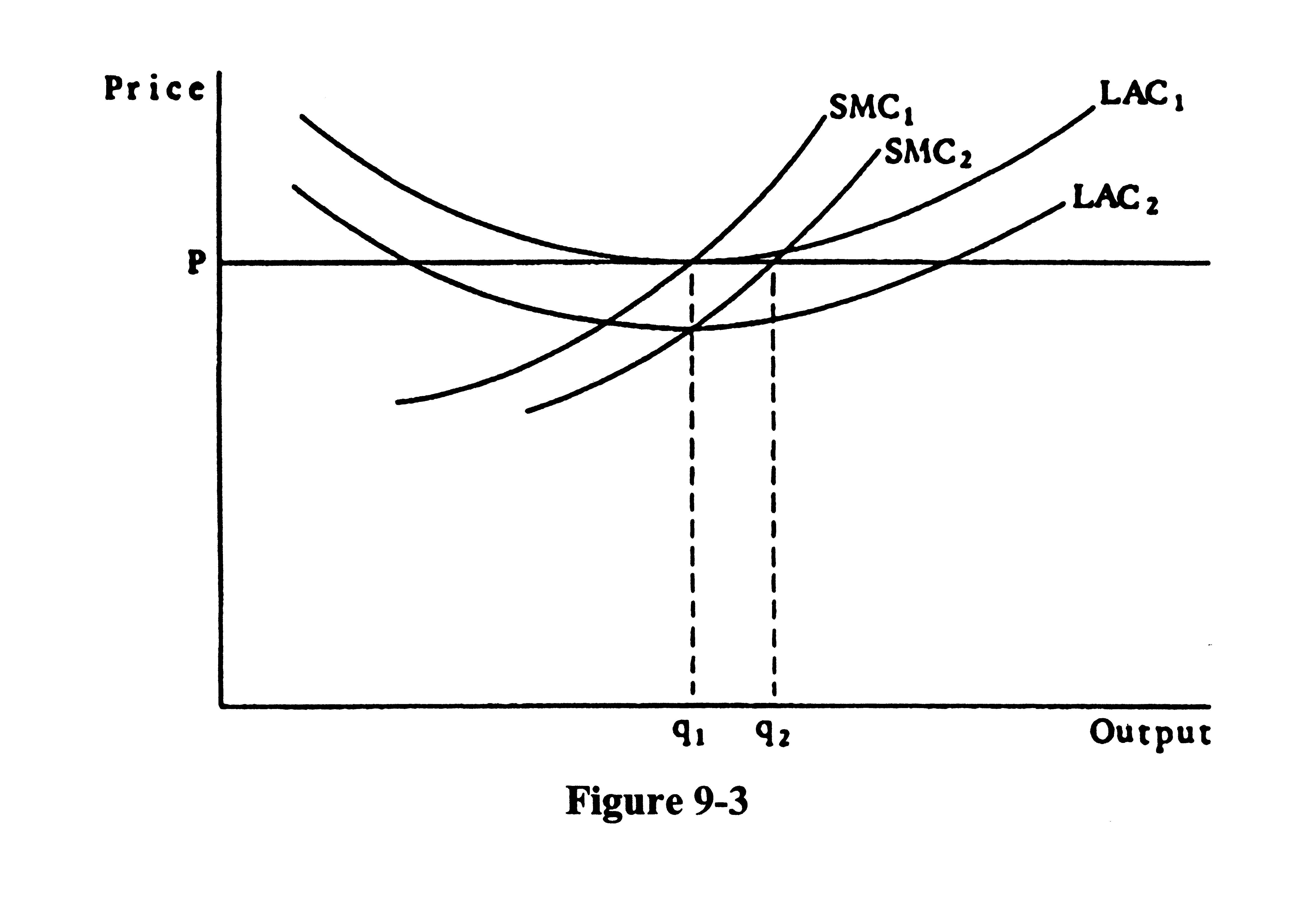
12. Figure 9-3 illustrates two firms in a competitive industry with different cost curves. How can this be a long-run equilibrium?
13. Explain how the shape of the long-run industry supply curve is determined.
14. Using two graphs, one for the firm and one for the industry, explain thoroughly how a competitive industry moves from one long-run equilibrium position to another.
15. Assume a new innovation is developed that reduces the cost of production for firms. What would be the effects on a competitive industry?
Questions 16 and 17 refer to Figure 9-4.
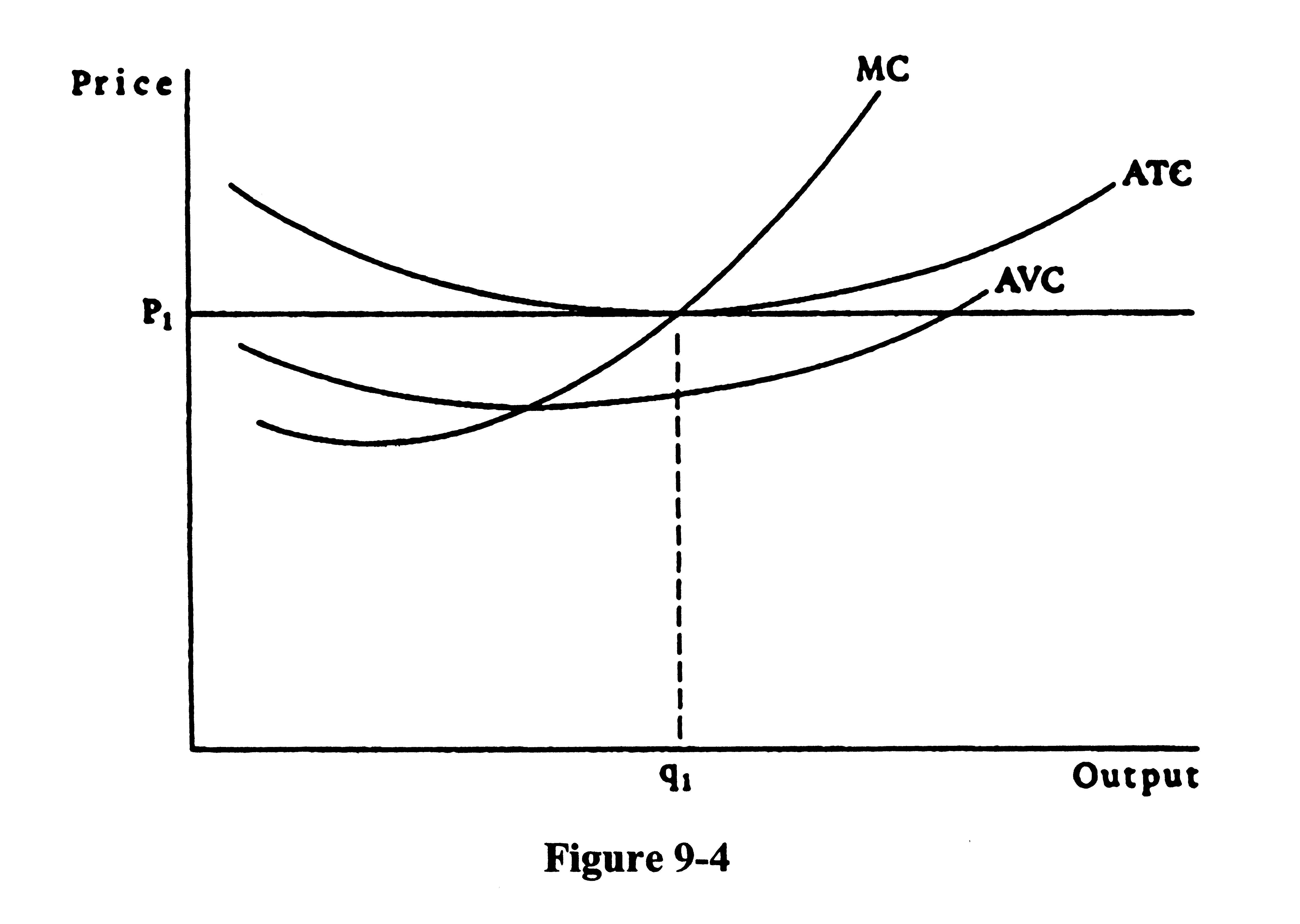
16. Suppose the price of the variable input increases.
a. What happens to the cost curves? Why?
b. What will happen to the quantity produced by the firm? Why?
c. Will the firm still operate in the short run? Explain.
17. Suppose the price of a fixed input increases.
a. What happens to the cost curves? Explain.
b. What will happen to the quantity produced? Why?
18. Suppose there is a market composed of 1,000 individuals with identical demand schedules and 100 firms with identical cost schedules. An individual's monthly demand schedule is given below. The cost relations are:
TC = 36 + 3.8q + 0.0lq2 MC = 3.8 + 0.02q
| Demand | |||
| (1) | (2) | (3) | (4) |
| Q | P | QD | QD |
| 1 | $7.00 | ||
| 2 | 6.60 | ||
| 3 | 6.20 | ||
| 4 | 5.80 | ||
| 5 | 5.40 | ||
| 6 | 5.00 | ||
| 7 | 4.60 | ||
| 8 | 4.20 | ||
| 9 | 3.80 | ||
| Supply | ||||
| (5) | (6) | (7) | (8) | (9) |
| qf | MC | Qs | MC | Qs |
| 90 | ||||
| 80 | ||||
| 70 | ||||
| 60 | ||||
| 50 | ||||
| 40 | ||||
| 30 | ||||
| 20 | ||||
| 10 | ||||
a. Fill in columns, 3, 6, and 7.

b. Find the market equilibrium price and level of output. Draw the market demand and supply curves in Figures 9-5(a).
c. Find the equilibrium price and level of output for the firm. Draw the firm's demand and cost curves in Figure 9-5(b). What are the firm's profits?
d. Is this a short-run equilibrium or a long-run equilibrium? How do you know?
e. Suppose 600 more people enter the market. Fill in the new market demand schedule in column 4. What is the new short-run equilibrium price and level of output for the market and for the firm? What are the profits for the firm? Add the relevant supply and demand curves to the graphs.
f. Suppose this is a constant-cost industry. What are the new long-run equilibrium prices and levels of output for the firm and the market? Where did the extra output come from?
g. Suppose, instead, that this is an increasing-cost industry, and the new cost relations for the firms are TC = 36 + 4.4q + 0.01q2 and MC = 4.4 + 0.02q. Fill in columns 8 and 9. What are the new long-run equilibrium price and levels of output for the firm and the market? (Hint: Average cost is at a minimum at 60 units.)
h. What causes the differences in the long-run equilibriums in parts f and g?
i. Return to the original long-run equilibrium in part a. Suppose costs change such that TC = 36 + 4.4q + 0.0lq2 and MC = 4.4 + 0.02q. What are the new short-run equilibrium price and levels of output for the firm and the market? What are the profits for the firm?
j. Suppose this is a constant-cost industry. What are the new long-run equilibrium price and levels of output for the market and for the firm?
The following questions relate to the material in Section 9.10: The Mathematics behind Perfect Competition.
19. The total cost function of a firm is TC = 10 + 2Q - 0.2Q2 + 0.01Q3
The price is $6.
a. What is the marginal cost function of the firm?
b. What are the total cost, average variable cost, and the average total cost functions of the firm?
c. What are the fixed costs of the firm?
d. What is the profit-maximizing level of output? What are the profits? How do you know the level of output maximizes profits instead of minimizes profits?
e. What is the lowest price for which the firm will produce in the short run?
SOLUTIONS
True/False
1. True
2. False
3. True
4. True
5. False
6. False. If P < AVC it will shut down.
7. True
8. True
9. True
10. True
11. False
12. True
13. True
14. True
15. True
Multiple Choice/Short Answer
1. c
2. d
3. d
4. c
5. d
6. a
7. Zero
8. q4
9. Zero
10. q2
11. d
12. a
13. c
14. c
15. b
16. a
17. c
18. d
19. a
20. c
21. d
22. d
23. d
24. a
25. b
Discussion Questions and Problems
1. a. 1. Large number of buyers and sellers ensures that no single buyer or seller can unilaterally affect price.
2. Unrestricted mobility of resources ensures the zero-profit condition of long-run equilibrium.
3. Homogeneous product allows us to define the industry easily and helps ensure price-taking behavior since the output of all firms is identical.
4. Possession of all relevant information ensures that one price prevails in the market and that individuals know which industries are profitable and which are not.
b. The assumptions are fairly realistic for some elements of agriculture.
c. Yes. The important point is how well the model explains and predicts and not the realism of its assumptions.
2. A demand curve relates price and quantity demanded. Total revenue equals (P)(Q)while average revenue equals price. A demand curve is also an average revenue curve since it equals the price at every quantity. A competitive firm's demand curve is its marginal revenue curve because it is horizontal. Thus, the change in total revenues from selling one more unit will always equal price.
3. a. Zero. Price is below the minimum point of AVC. The firm is losing $500.
b. 220 bushels of wheat. At this level of output, P = MR = MC so profits are being maximized. The firm is losing $380.60 (TR = 220 x $1.67 = $367.40 and TC = $750). Note that the loss is less than the $500 loss when the firm shuts down.
c. 250 bushels of wheat. P = MR = MC at this level of output. The firm is making $400 in profits (TR = 250 x $5 = $1250 and TC = $850).
d. The shutdown point is the minimum point of the AVC curve, which lies between 100 and 150 bushels of wheat
e. When price is below AVC, output is zero and there is no relationship between price and output. When price is above the minimum point of the AVC curve, then output expands as price increases because of the shape of the MC curve.
4. The firm should produce where MR = MC. If MR > MC the firm can increase profits by producing one more unit because the addition to total revenue from producing the unit is greater than the addition to total costs. If MR < MC the firm can increase profits by producing one less unit because the reduction in total revenue from not producing the unit is less than the reduction in total costs. Since the firm can increase profits by increasing output whenever MR > MC and by reducing output whenever MR < MC, profits are at a maximum when MR = MC. Of course, this applies only if P > AVC or the firm will shut down. Note, too, that for a competitive firm P = MR so the rule can be stated P = MC.
5. A firm will go out of business in the long run if it cannot cover all of its costs. These costs include the implicit costs of the inputs supplied by the owners of the firm. The return on these inputs is greater elsewhere so the owners will liquidate the firm and move these inputs to industries where the return is greater.
6. Output
Price (bushels of wheat)
$ 1.00 15,000
1.25 19,000
1.67 22,200
2.50 24,000
5.00 25,000
10.00 25,500
The industry supply curve is upward sloping because the MC curves of the firms are upward sloping due to the law of diminishing marginal returns.
7. The average cost curves will tell us whether the firm is making profits, but this is irrelevant to the determination of price and output in the short run. The supply curve of the industry is found by summing horizontally the supply curves of the firms. The firm's supply curve is its MC curve above AVC. Thus the firm will produce where its supply curve intersects its demand curve because at that point P = MC.
8. Total costs include all opportunity costs, including the opportunity costs of the owners. Hence, if revenues cover all these costs, the owners couldn't do better anywhere else.
9. The durable assets are used in other industries. This process may involve modifying the assets to some extent. If a particular input is so specialized that it cannot be used in other industries, it will be scrapped.
10. Yes. Fixed costs are the costs that do not vary with output, but they can change. For example, the property tax on a plant can change.
11. a. 240 bushels of wheat. Firm uses 6 tons of fertilizer. It is losing $200.
(TR = $2.50 x 240 = $600. TC = $800).
b. 250 bushels of wheat. The firm uses 7 tons of fertilizer. It is losing $50. (TR = $2.50 x 250 = $625. TC = $675.)
c. No. If the new price of fertilizer applies to all firms in the industry, the changes in output by all firms will cause a change in price and a new short-run equilibrium.
12. This can be a long-run equilibrium if Firm 2 (with LAC2) has some inputs that are more efficient than those of Firm 1. Then Firm 2's costs curves do not reflect the opportunity cost of the more efficient inputs. When the opportunity costs of these inputs are calculated, the LAC2 curve will shift upward to the LAC1 curve.
13. The shape of the long-run industry supply curve is determined by the shape of the input supply curves. If the input supply curves are horizontal, then costs will not change as new firms enter the industry. The result is a constant-cost industry with a horizontal long-run supply curve. If the supply curves shape upward, it is an increasing-cost industry and the long-run supply curve is upward sloping. If the input supply curves slope downward, it is a decreasing cost industry and the long-run supply curve is downward sloping.
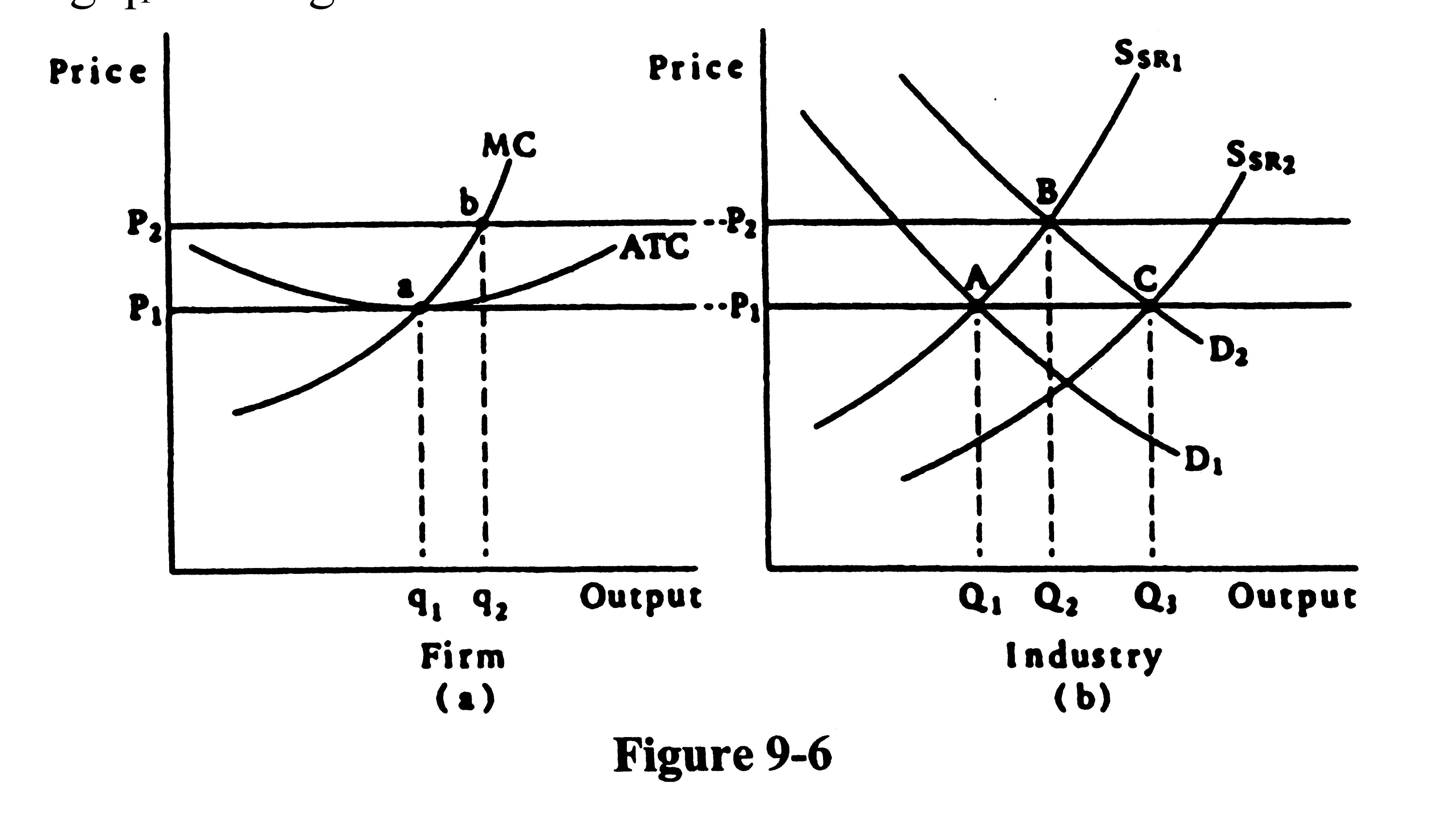
14. A competitive industry is in long-run equilibrium when all firms are making zero profits. In Figure 9-6 (b), this is point A. In Figure 9-6 (a), it is point a. If demand increases to D2, price increases to P2. In the short run, each firm moves along its MC curve until P = MC. This is point b in Figure 9-6 (a), with output q2. Each firm in the industry is now making economic profits. As we move to the long run, new firms enter the industry. As they enter, industry output increases and price falls. If this is a constant-cost industry, new firms will enter until price falls all the way back to P1. The new short-run supply curve intersects D2 at point C. The price facing each firm is P1 so all firms are now making zero profits (point a). The increase in industry output from Q1 to Q3 is supplied by new firms since all firms originally in the industry are producing q1 units again.
15. The cost curves of firms shift downward, which means that the firms are now making profits. The profits will attract new entrants and encourage existing firms to expand output. The increased industry output causes price to fall until all firms are making zero profits once again.
16. a. They shift upward because costs are higher at every level of output.
b. The quantity produced by the firm will decrease. Since MC shifts upward and price remains constant, the new level of output where P = MC will be to the left of q1.
c. It may or may not depending on how much the curves shift upward. If price is above AVC, the firm will produce, but if the AVC curve shifts up so much that its minimum point is above P1, the firm will shut down.
17. a. The ATC curve shifts up but the AVC and MC curves do not shift because fixed costs do not affect variable costs.
b. Quantity produced will not change since MC did not change. The firm will now make losses in the short run because the ATC curve shifted upward, though.
18.
| Demand | |||
| (1) | (2) | (3) | (4) |
| Q | P | QD | QD |
| 1 | $7.00 | 1,000 | 1,600 |
| 2 | 6.60 | 2,000 | 3,200 |
| 3 | 6.20 | 3,000 | 3,200 |
| 4 | 5.80 | 4,000 | 6,400 |
| 5 | 5.40 | 5,000 | 8,000 |
| 6 | 5.00 | 6,000 | 9,600 |
| 7 | 4.60 | 7,000 | 11,200 |
| 8 | 4.20 | 8,000 | 12,800 |
| 9 | 3.80 | 9,000 | 14,400 |
| Supply | ||||
| (5) | (6) | (7) | (8) | (9) |
| qf | MC | Qs | MC | Qs |
| 90 | $5.60 | 9,000 | $6.20 | 9,000 |
| 80 | 5.40 | 8,000 | 6.00 | 8,000 |
| 70 | 5.20 | 7,000 | 5.80 | 7,000 |
| 60 | 5.00 | 6,000 | 5.60 | 6,000 |
| 50 | 4.80 | 5,000 | 5.40 | 5,000 |
| 40 | 4.60 | 4,000 | 5.20 | 4,000 |
| 30 | 4.40 | 3,000 | 5.00 | 3,000 |
| 20 | 4.20 | 2,000 | 4.80 | 2,000 |
| 10 | 4.00 | 1,000 | 4.60 | 1,000 |
a. See schedule above.
b. QD = QS = 6,000 units at a price of $5.00. See Figure 9-7.
c. P = MC at $5.00. qf = 60 units. See Figure 9-7. Profits = TR - TC =
pqf - 36 - 3.8q - 0.0lq2 = $5.00(60) - 36 - 3.8(60) - 0.01(602) = 300 - 36 - 228 - 36 = 0.
d. This is a long-run equilibrium because each firm is making zero profits.
e. Market price is $5.40 where Q'D = QS = 8000 units. The firm faces a price of $5.40, and each firm produces 80 units. Profits = $5.40(80) - 36 - 3.8(80) - 0.01(802) = 432 - 36 - 304 - 64 = $28. See Figure 9-7.

f. P = $5.00; QD = QS = 9,600 units; qf = 60 units. Sixty new firms entered the market.
g. Since average costs are minimized at 60 units, long-run equilibrium exists at 60 units and P = AC = MC at 60 units of output. Marginal costs for 60 units are MC = 4.4 + 0.02(60) = $5.60. Therefore, equilibrium price must be $5.60. Quantity demanded at $5.60 is 7,200 units. If each firm produces 60 units, there must be 120 firms.
h. The long-run supply curve is horizontal in part f but is upward sloping in part g because the increased demand for inputs in part g causes the prices of inputs to increase. Consequently, costs rise and the long-run supply curve is upward sloping.
i. We must find the quantity demanded, QD, in column 3 equal to the quantity supplied, QS in column 9, where P = MC. This occurs at a price of $5.40 where QD = QS = 5,000 units. Each firm produces 50 units. Profits equal $11.
From part g we know minimum average cost is at 60 units. Therefore, MC = 4.4 + 0.02(60) = $5.60. Equilibrium price is at $5.60, and QD = 4,500 units. Each firm produces 60 units, so there are 75 firms. That is, 25 firms went out of business.
19. a. Marginal costs are found by taking the derivative of the total cost function
MC = (dTC/dQ) = 2 - 0.4Q + 0.03Q2
b. TVC = 2Q - 0.2Q2 + 0.01Q3
AVC = 2 - 0.2Q + 0.01Q2
ATC = (10/Q) + 2 - 0.2Q + 0.01Q2
c. $10
d. = TR-TC = $6Q - 10 - 2Q + 0.2Q2 - 0.01Q3
d/dQ = 6 - 2 + 0.4Q - 0.03Q2 = 0
0.03Q2 - 0.4Q - 4 = 0
Therefore, Q = 20 and profits are $70.
The second derivative of the total cost function is -0.4 + 0.06Q. When Q = 20, this is positive so 20 units is a maximum. (Note: the other solution to the quadratic is negative so it cannot be a maximum.)
e. The shutdown point in the minimum point of AVC.
d(AVC)/dQ = -0.2 + 0.02Q = 0
Therefore, the shutdown point is 10 units and price is $ 1.
209


