Microeconomics graphs and charts details and answers.
CHAPTER 11: Monopoly
CHAPTER 11
Monopoly
CHAPTER ANALYSIS
A monopoly is the sole producer of a good that has no close substitutes. Since it is the only producer of the good, the monopoly firm controls market price and quantity. Some industries are similar to monopolies in that only a few firms compete, and those that do have monopoly power to set price above marginal cost.
11.1 The Monopolist’s Demand and Marginal Revenue Curves
The monopolist's demand curve is the industry demand curve, and since industry demand curves slope downward, the monopolist's demand curve also slopes downward. The shape of the demand curve is the key difference between a competitive firm and a monopoly. This is because a competitive firm has a horizontal demand curve while a monopoly has a downward sloping demand curve. Monopoly firms are price makers, while competitive firms are price takers.
In Chapter 9 we saw that marginal revenue equals price for a competitive firm, and that the firm's demand curve is also its marginal revenue curve. However, for a monopoly the marginal revenue curve is different from the demand curve, and price does not equal marginal revenue. The reason for the difference is that the monopoly demand curve slopes downward, indicating that as price changes, quantity changes as well. Therefore, a change in total revenue comes from a change in both price and quantity. Table 11.1 in the text shows the relationship between a monopolist’s total and marginal revenue.
11.2 Profit-Maximizing Output of a Monopoly
The profit-maximizing level of output of any firm, competitive or monopoly occurs where marginal revenue equals marginal cost. Figure 11-1 illustrates the profit-maximizing level of output for the monopolist. Since MR = MC at Q1, Q1 is the profit-maximizing level of output. The price charged is found by identifying the price on the demand curve for which Q1 can be sold. At output Q1 the firm can charge a price of P1. Note that a monopoly will not necessarily be profitable. Figure 11-1 shows four average cost curves, and each is permissible since the marginal cost curve intersects each average cost curve at its minimum. If AC2 applies, profits are equal to the area P1ABC. However, if AC3 applies, the firm earns zero profits, while if AC4 applies; the monopolist operates at a loss. If AC4 are long-run costs, the monopolist will go out of business. Note that the profit-maximizing level of output is the same because the marginal cost curve is the same for each.

The monopoly price is related to the price elasticity of demand. It can be shown that the gap between price and marginal cost is inversely related to the price elasticity of demand. That is:
(P - MC)/P = 1/ or P = MC/(1-(1/)).
Therefore, if the monopolist knows its price elasticity of demand and its marginal cost, it can calculate its profit maximizing price.
The above expression also shows that the price markup is equal to the inverse of the existing price elasticity of demand. When demand is relatively inelastic, the price markup will be greater than for cases when demand is relatively elastic.
11.3 Further Implications of Monopoly Analysis
There are six additional points regarding demand, marginal revenue, profit, and elasticity that need to be addressed. First, while the monopolist faces a downward sloping demand curve, it does not have a supply curve. This is because the monopolist is a price maker and the price it charges solely depends on demand, marginal revenue, and marginal costs.
Second, it is definitely possible for a monopolist to make zero or even negative profits. Monopolists are usually viewed as making very high profit but this is not always the case. If its long run average total cost curve lies above the demand curve, profit will be negative. Third, the monopolist’s demand curve is elastic where marginal revenue is positive. When demand is elastic, a percentage decrease in the price leads to a greater percent increase in quantity demanded. This means total revenue is increasing, which implies marginal revenue is positive.
Fourth, when marginal revenue is equal to zero, total revenue is maximized and the demand curve is unit elastic. When demand is unitary elastic, a percentage decrease in the price leads to an equal percentage increase in quantity demanded. Therefore, there is no change in total revenue, implying marginal revenue is constant.
Fifth, when marginal revenue is less than zero, total revenue is falling and demand is inelastic. When demand is relatively inelastic, a percent decrease in price leads to a greater percent decrease in quantity, which therefore implies total revenue is decreasing and marginal revenue is negative.
Finally, the price charged by a monopolist is always on the elastic portion of the demand curve. This is because we know a monopolist maximizes profit by choosing output where marginal revenue is equal to marginal cost. Since marginal costs are always positive, marginal revenue must also be positive at the profit maximizing level of output.
11.4 The Measurement and Sources of Monopoly Power
Pure monopoly is rare, but many firms may face downward-sloping demand curves. Any firm that faces a downward-sloping demand curve has some monopoly power. A measure of this monopoly power is the Lerner index:
Lerner index = (P - MC)/P.
We have already seen that this ratio equals the inverse of the elasticity of demand. Hence, the more elastic the demand curve, the lower the Lerner index, which means the price markup is relatively low. In the extreme, a perfectly elastic demand curve would have a Lerner index equal to zero, indicating no monopoly power.
The extent of monopoly power is determined by the elasticity of the market demand curve and the elasticity of supply of other firms. The monopoly power of a firm will be greater if there are barriers to entry that keep out new firms. A barrier to entry is a factor that limits the number of firms operating in a market. Recall that under perfect competition, profits provide an incentive for new firms to enter an industry. In the case of monopoly, barriers to entry may prevent or retard the entry of new firms, enabling the monopolist to continue making profits in the long run.
The authors identify four categories of entry barriers:
Absolute cost advantage--the long-run average total cost of the incumbent firm is below that for rivals or potential entrants. This can be due to access to unique resources or more productive resources. For example, diamond mines are a necessary input to the production of diamonds. Since DeBeers Company owns most of the mines, they have an absolute cost advantage in the production of diamonds.
Economies of scale—a situation where the firm can increase output more than proportionally to its input costs. As a result, the monopolist faces a declining long-run average cost curve which leads to a natural monopoly. A natural monopoly is when production cost is minimized if one firm supplies the entire output.
Product differentiation—this is when consumers perceive a product as superior to those offered by potential rivals. For example, some consumers may feel this way towards goods such as Nike brand shoes, Kleenex tissues, Pudue chicken, etc.
4. Regulatory barriers--the government grants patents, copyrights, franchises and licenses to firms that often prevent other firms form entering the industry. For example, a patent on a pharmaceutical drug gives the company exclusive ownership rights for 17 years.
11.5 The Efficiency Effects of Monopoly
The existence of a monopoly leads to an inefficient mix of output because consumers would be better off if more was produced at a lower price. In other words, the positive profit earned by a monopolist represents a cost to society. In order to examine the efficiency effects of a monopolist, we will compare it to the polar opposite industry, perfect competition.
Perfect competition and monopoly differ in several important ways. First, P = MC under perfect competition, while P > MC under monopoly. Remember, the long run output in perfect competition is where P = MC = MR. Second, for a monopolist, average total cost is not minimized at the profit maximizing output. In perfect competition, price always is equal to the minimum point on the firm’s average total cost curve in the long run. Third, it is possible for a monopolist to make positive profit in both the short run and long run. Perfectly competitive firms can only make positive profit it in the short run. In the long run, entry reduces profit to zero. Fourth, a monopolist restricts output and charges higher prices. This represents a welfare cost to society. Fifth, the price output combination associated with a monopolist creates a deadweight loss. This is because the high prices result in a gain in consumer surplus that is outweighed by the loss in consumer surplus. Therefore, the high prices create a net loss to society. An example depicting deadweight loss is shown by Figure 11.9 in the text.
The welfare costs discussed above represent an example of static analysis. This type of analysis examines efficiency effects at one point in time. On the other hand, dynamic analysis looks at efficiency of a market over time. Dynamic analysis suggests that the social costs of a monopoly may not be as great as suggested by static analysis. In other words, when examining a monopoly over time generates positive welfare effects. For example, monopolies often introduce new products and new innovations because the existence of patents and copyrights gives them incentive to do so. Also, in order to increase profit, monopolists many times attempt to find ways to lower production costs. Therefore, when analyzing a monopoly, it is important to do so from both a static and dynamic perspective.
11.6 Public Policy towards Monopoly
The U.S. policy toward a monopoly has largely relied on static analysis. The primary way in which the U.S. government regulates monopolies is through antitrust laws. These laws include a series of codes and amendments to promote a competitive environment. The three major statutes of antitrust law include the Sherman Act, the Clayton Act, and the Federal Trade Commission Act.
The Sherman Act, passed in 1890, declared restraints on trade and monopolies to be illegal. This act was broadly written which created many problems with its interpretation. As a result, the Clayton Act and Federal Trade Commission Act were both passed in 1914. The Clayton Act explicitly outlawed specific acts such as predatory pricing and price discrimination. The Federal Trade Commission Act created the Federal Trade Commission which is an agency that has the authority to enforce and prohibit unfair methods of competition.
In addition to antitrust laws, the U.S. government also relies on price regulation. As applied to a monopolist, price regulation basically sets price ceilings on regulated firms. Since a monopoly increases price by restricting output, a price ceiling has the effect of eliminating the incentive to restrict output. In Figure 11-2 (figure missing), the unregulated monopolist would charge $15 and produce 600 units per month. If the government would set a price ceiling of $12, the monopoly would produce the perfectly competitive (efficient) level of output. This result is due to the effect of the price ceiling. A price ceiling of $12 means that the firm can sell as many units as it wants (up to 1,000 units) at a price of $10. To sell more than 1,000 units, the firm would have to charge a price less than $12. The price ceiling essentially changes the monopolists downward sloping demand curve to a horizontal demand curve, at least out to 1,000 units. Its demand curve becomes FBD and its marginal revenue curve becomes FBGMR. The monopolist maximizes profits by producing the level of output where marginal cost equals marginal revenue, which is a level of output of 1,000 units and a price of $12which is the competitive price-output combination.
11.7 The Math behind Monopoly (online only content)
This section uses mathematical analysis to confirm two major conclusions addressed in the text. These include the relationship between a monopolist’s demand and marginal revenue curves, and the monopolist’s optimal output choice.
First, we examine the relationship between the monopolist’s marginal revenue and demand curve is discussed. Total Revenue is equal to price times quantity:
R = PQ.
Since we are dealing with market demand, price is an inverse function of output where:
P = f(Q) and dP/dQ < 0.
Marginal revenue is the derivative of total revenue with respect to Q:
dR/dQ = MR = P + Q(dP/dQ).
Marginal revenue is always less than price for a downward sloping demand curve since P is positive and dP/dQ is negative.
Factoring out P, we can see the relationship between price, marginal revenue, and price elasticity of demand:
MR = P[1+ (Q/P)(dP/dQ)];
= P(1 - (1/η)).
The second major conclusion we mathematically examine is the profit maximization choice for the monopolist. Profit is equal to:
π = R – C.
In the above equation, π is profit, R is revenue, and C is total cost. All of these variables are a function of output.
The first order condition for maximizing profit is to take the first derivative with respect to output and set it equal to zero:
dπ/dQ = (dR/dQ) – (dC/dQ) = 0.
The equation above shows that marginal revenue is equal to marginal cost when profits are maximized.
An alternative way to show the profit maximizing condition as it relates to all types of firms is shown below. Expressing revenue as price multiplied by quantity gives:
π + PQ – C.
Taking the first derivative with respect to output, we get:
dπ/dQ = P + Q(dP/dQ) – (dC/dQ) = 0.
Therefore, if the firm is a monopoly, marginal revenue must equal marginal cost. If the firm is competitive, dP/dQ equals zero, and the equation reduces to the profit maximizing rule. Note that price will be above marginal cost at the monopoly profit maximizing equilibrium.
ILLUSTRATIONS
The market for presidential candidates offers an example of barriers to entry. The two dominant “firms” in presidential politics are the Democratic and Republican parties. In 1980, Jimmy Carter was the Democratic candidate and Ronald Reagan the Republican. John Anderson entered the race as an independent candidate.
As representatives of their parties, Carter and Reagan were automatically on the ballots of all the states. Since Anderson was an independent, he was not on all of the ballots. In order to get his name on the ballot, he had to initiate petition drives in many states and court challenges in others. This activity required the use of funds that neither Carter nor Reagan had to spend. Further, Carter and Reagan received matching funds from the government, while Anderson had to obtain a minimum percentage of the vote in order to receive matching funds. Carter and Reagan were assured of equal time on TV and radio under the Fairness Doctrine, which did not apply to Anderson. Further, Anderson was not included in the nationally televised debates. It is more costly for an independent entrant to run for president than for representatives of the established parties because of various legal restrictions. Thus there are substantial barriers to entry in the market for president.
The 1992 and 1996 Ross Perot was a third-party candidate. Perot did better than any third-party candidate in the history of the country. He was included in the debates, and received considerable press coverage. He also had the financial resources to ensure he was on the ballots in all the states. Barriers to entry, though substantial, do not always mean that entry cannot take place at all.
The 2000 election illustrated barriers to entry again. Pat Buchanan represented Ross Perot's party, the Reform Party, and Ralph Nader represented the Green Party. Neither candidate was included in the televised debates, which is a serious drawback for a third-party candidate.
The Aluminum Company of America
The Aluminum Company of America (ALCOA) was the sole domestic manufacturer of aluminum ingots from the late 1800s until World War II. Initially, the monopoly position of the firm was due to patents. When the patents expired in the early 1900s, ALCOA maintained its monopoly position by controlling the sources of the key input into the manufacturing process-bauxite. ALCOA signed long-term contracts with owners of bauxite supplies that guaranteed that they would sell only to ALCOA. These contracts were declared invalid by the courts in 1912. After 1912, ALCOA maintained its dominant position by quickly acting to meet any increases in demand with new capacity to produce aluminum. After World War II, ALCOA's position declined as new firms entered the market, aided by a government antitrust suit against ALCOA, the disposal of government-controlled aluminum plants during the war, and rapidly increasing demand for aluminum after the war.
KEY CONCEPTS
monopoly product differentiation
monopoly power regulatory barriers
price maker Lerner index
barriers to entry deadweight loss
absolute cost advantages static analysis
economies of scale dynamic analysis
natural monopoly antitrust laws
REVIEW QUESTIONS
True/False
1. The sole producer of a good can charge whatever price it wants.
2. When a demand curve slopes down, marginal revenue is always less than price.
3. A monopoly produces where P = MC.
4. The more elastic the demand, the closer price is to marginal revenue.
5. The supply curve of a monopoly is upward sloping.
6. Monopolies always earn economic profits.
7. Marginal revenue equals zero when the demand curve has an elasticity of one.
8. For monopoly to exist, entry barriers must exist.
9. The possibility of entry by new firms constrains the exercise of monopoly power.
10. For the same market demand and cost conditions, price is higher and output is lower under monopoly than under perfect competition.
11. The desire to make monopoly profits is a spur to innovation.
12. As in perfect competition, a price ceiling in monopoly leads to reduced output.
Multiple Choice/Short Answer
1. A monopolist's marginal revenue curve lies below its demand curve because
a. the average revenue curve is constant as quantity increases.
b. the change in total revenue is constant as quantity increases.
c. a monopoly does not have a supply curve.
d. the demand curve slopes downward.
Questions 2 to 5 refer to Figure 11-3.
2. If MC = 0, what is the profit maximizing level of output?
3. The demand curve is elastic
a. over the range AB.
b. over the range EB.
c. at point E.
d. over the range BC.
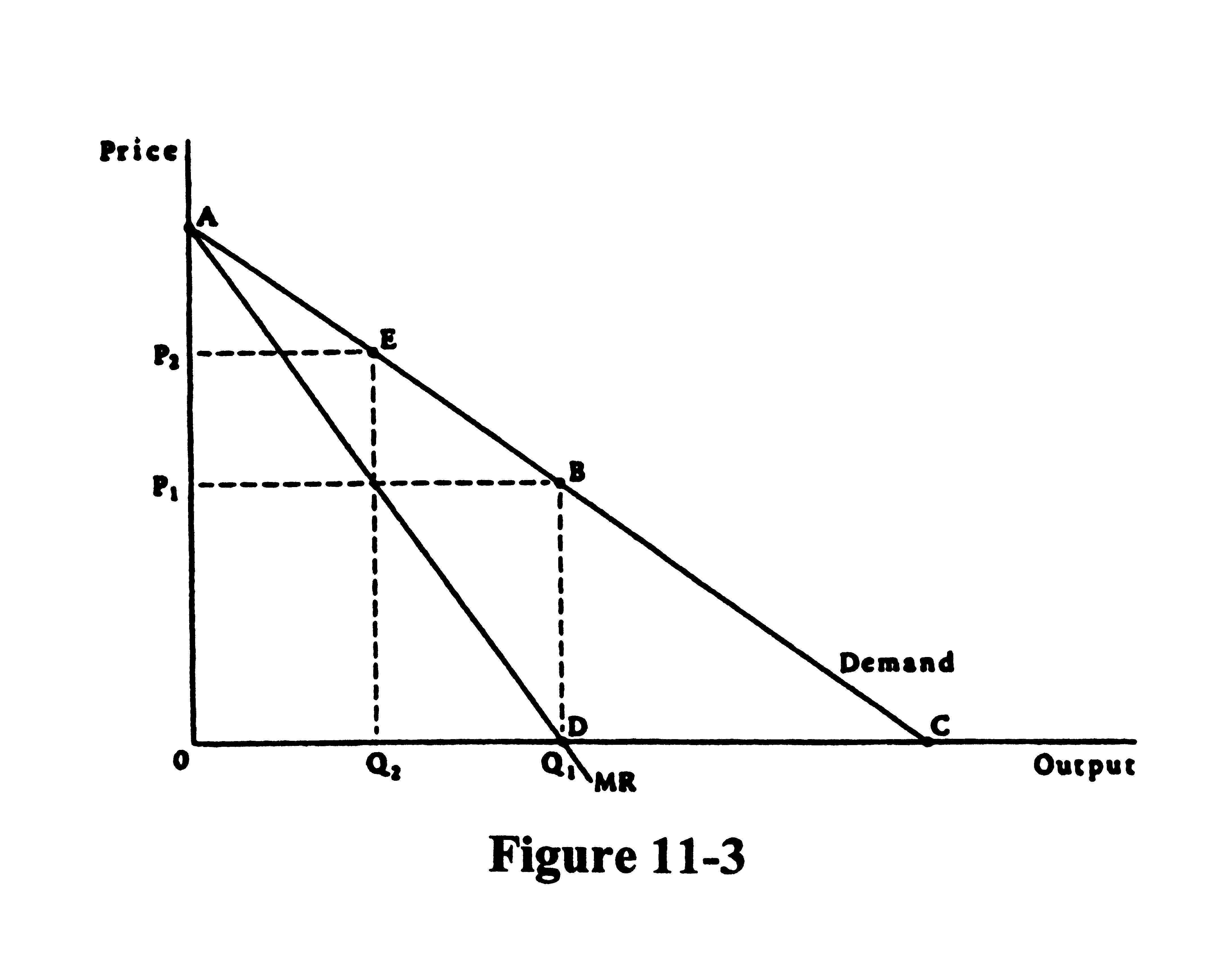
4. The demand curve is inelastic
a. over the range AB.
b. at point B.
c. over the range EC.
d. over the range BC.
5. The demand curve is unit elastic
a. over the range AB.
b. at point E.
c. at point B.
d. over the range RC.
6. a. What is the price elasticity of demand when price is twice as large as marginal revenue?
b. What is the price elasticity of demand when P = $20 and MC = $15?
7. If marginal revenue is greater than marginal cost, a monopolist will
a. raise price.
b. decrease output.
c. increase output.
d. shutdown.
Questions 8 to 11 refer to Figure 11-4.

8. What price will a profit-maximizing monopolist charge?
9. The profits of the firm are measured by the area
a. P2GQ3O.
b. P1BEP3.
c. P1BCP2.
d. BCG.
10. The supply curve of the firm
a. is the MC curve.
b. is the MC curve that lies above point F.
c. is the AC curve to the right of F.
d. does not exist.
11. The welfare cost of monopoly is measured by the area
a. ABP1.
b. ABCP2.
c. BGC.
d. P1BGP3.
12. The Lerner index is
a. P > MC.
b. (P - MC)/P.
c. (MR - MC)/P.
d. P(1 - 1(1/)).
13. A natural monopoly exists due to
a. the control of a key input.
b. a downward sloping long-run average cost curve.
c. the government's granting the firm a monopoly.
d. entry lags.
14. Suppose the monopolist in Figure 11-5 knows that new firms will enter at any price above $17. What output will it produce?
a. Q1
b. Q2
c. Q3
d. 0

15. The deadweight loss of monopoly is due to the fact that
a. monopolists are greedy.
b. monopolies earn economic profits.
c. monopolies restrict output in order to raise price.
d. a monopoly does not produce at the minimum point of its average cost curve.
16. Economic profits of a monopoly represent
a. a transfer of income from consumers to producers.
b. the inefficiency of monopoly.
c. welfare cost of monopoly.
all of the above.
A firm is observed making monopoly profits. Using dynamic analysis of monopoly, one would argue that
the firm is inefficient and should be dealt with by antitrust or regulatory authorities.
the firm's profits should be taxed away.
the monopoly profits are not a concern as long as the firm is producing where P = MC.
the profits are a reward for successfully developing a new product and the firm should not be dealt with by antitrust or regulatory authorities.
18. Dynamic analysis of monopoly
a. reinforces static analysis in condemning the effects of monopoly.
b. offers little difference from static analysis of monopoly.
c. suggests that the welfare effects of monopoly are not as bad as static analysis suggests.
d. indicates that monopolies always are beneficial on net to society.
Questions 19 and 20 refer to Figure 11-6.
19. If the government forces the monopolist to lower price from P1 to P2, the monopolist will change its output from Q4 to
a. Q1.
b. Q2.
c. Q5.
d. Q6.
20. If the price is set at P3, output will be
a. Q3.
b. Q6.
c. Q7.
d. Q9.

Discussion Questions and Problems
1. Explain why the marginal revenue curve lies below the demand curve.
2. a. Fill in the following table:
| Price | Quantity Sold | Total Revenue | Marginal Revenue | Price Elasticity |
| $22 | ||||
| 20 | ||||
| 18 | ||||
| 16 | ||||
| 14 | ||||
| 12 | ||||
| 11 | 5.5 | |||
| 10 | ||||
| 10 |
b. If marginal costs were constant at $8, how much output would be produced by a perfectly competitive industry? How much by a monopolist?
c. If marginal costs were constant at $4, how much would be produced under perfect competition? Would the industry be on the elastic or inelastic portion of its demand curve? How much would be produced under monopoly? Is the monopoly on its elastic or inelastic portion of its demand curve?
3. Refer to Discussion Problem 18 in Chapter 9 of the Study Guide to solve this problem. Suppose the following holds true: the firms merge and became a monopoly, the government prevents new firms from entering the industry, and the monopolist's marginal cost curve is identical to the supply curve of the perfectly competitive industry.
a. Fill in the following table:
| Price | Quantity Sold | Total Revenue | Marginal Revenue |
| $7.00 | 1,000 | ||
| 6.60 | 2,000 | ||
| 6.20 | 3,000 | ||
| 5.80 | 4,000 | ||
| 5.40 | 5,000 | ||
| 5.00 | 6,000 | ||
| 4.60 | 7,000 | ||
| 4.20 | 8,000 | ||
| 3.80 | 9,000 |
b. What output will the monopolist produce? What price will the monopolist charge? By how much does the monopolist restrict output?
c. Is the monopolist on the elastic portion of its demand curve? How do you know?
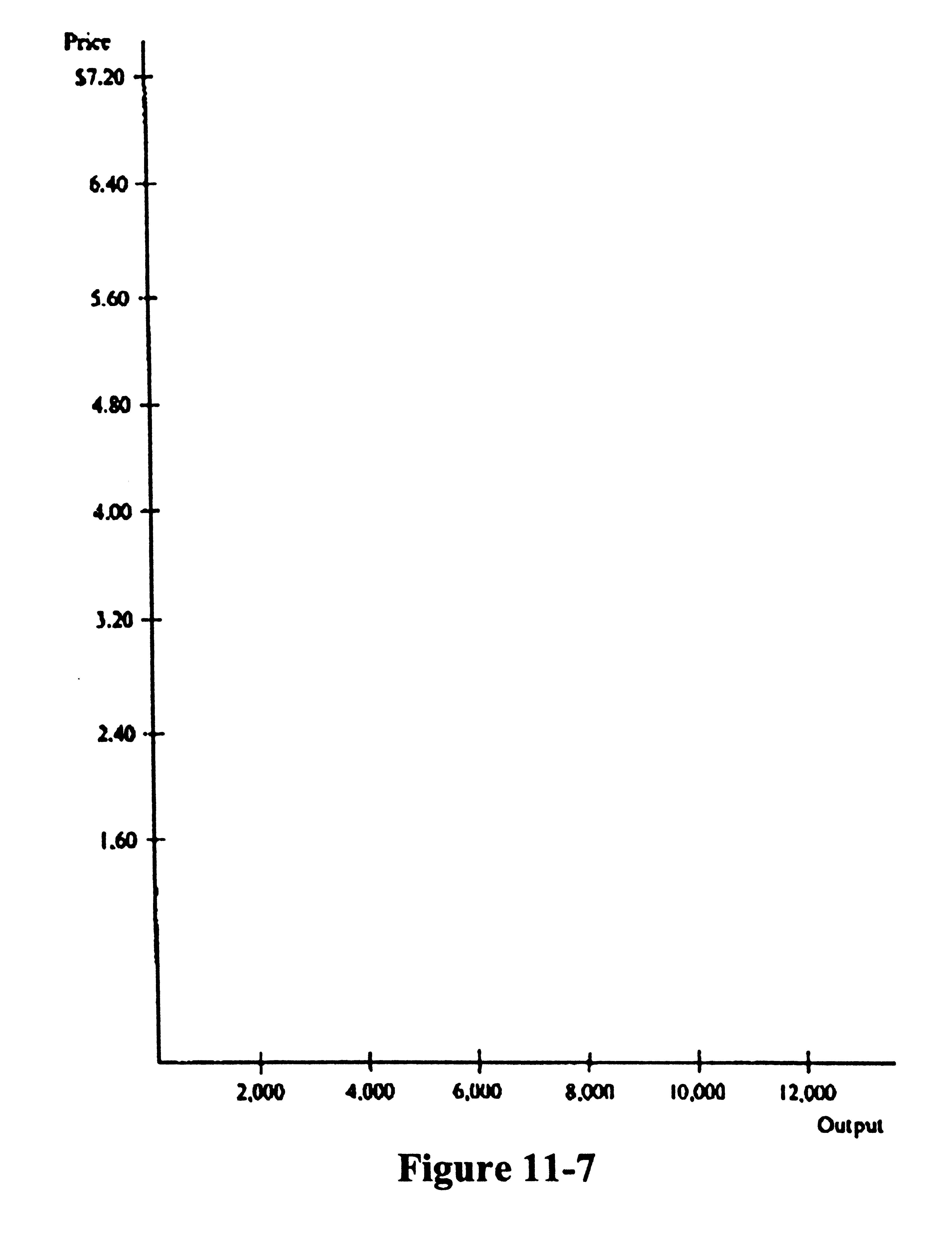
d. In Figure 11-7, draw the monopolist’s demand curve, marginal revenue curve, and marginal cost curve. Be sure to label the equilibrium point
e. Suppose demand goes up as in part e of Problem 18 in Chapter 9. Draw the new demand curve and the new marginal revenue curve. What is the new short-run price and quantity?
f. What will happen in the long run?
g. What are the long-run effects if the government did not block entry when the firms merged?
4. a. Suppose marginal cost of gasoline is $1.00, and an isolated gasoline station in Nevada has a price elasticity of demand for gasoline of 2. What price will the station charge for gasoline?
b. What is the Lerner index?
5. Explain why a monopolist does not have a supply curve.
6. "Demand is infinitely elastic in perfect competition, so the more elastic the demand the more the firm is like a competitive firm. Therefore, if a firm has an elastic demand, it is not a monopoly." Do you agree or disagree and why?
7. A monopolist produces on the elastic portion of its demand curve, which suggests that the monopolist would rather lower price than raise price since total revenue increase when price is reduced. Why would we never observe a monopolist raising price?
8. "The more narrowly a market is defined, the more likely a firm will be considered a monopoly." Do you agree or disagree, and why?
9. In the early 1900s, U.S. Steel owned the mines that produced the richest iron ore in the country. Was this a source of monopoly for U.S. Steel? Is U.S. Steel a monopoly today? Support your answer.
10. Will an unregulated monopolist always charge the price where marginal revenue equals marginal cost? Explain.
11. What is meant by monopoly power? How can firms that are not pure monopolies have monopoly power?
12. What is the source of the ill effects of monopoly? Explain.
13. Will perfect competition always result in more output and a lower price than monopoly? Explain.
14. How does dynamic analysis of monopoly differ from static analysis? How is this related to antitrust policy?
The following questions relate to the material in Section 11.7: The Math behind Monopoly.
15. Explain, mathematically, why P = MR under perfect competition and P > MR under monopoly.
16. The demand function for a monopolist is P = 30 - 0.75Q and total costs are TC = 20 + 9Q + 0.3Q2. What is the profit-maximizing level of output? What are profits? What would be the price and output under perfect competition if the monopolist's marginal cost curve is the competitive industry's supply curve?
SOLUTIONS
True/False
1. False
2. True
3. False
4. True
5. False. A monopoly does not have a supply curve.
6. False
7. True
8. True
9. True
10. True
11. True
12. False
Multiple Choice/Short Answer
1. d
2. Q1
3. a
4. d
5. c
6. a. 2
b. 4
7. c
8. P1
9. b
10. d
11. c
12. b
13. b
14. b
15. c
16. a
d
c
19. c
20. b
Discussion Questions and Problems
1. The demand curve slopes downward, which implies that the firm must lower price to sell additional units. This lower price applies to all units, however, and not just the additional units. The revenue earned on the output that could have been sold at a higher price falls as a result of the lower price. This reduction in revenue offsets, to a degree, the addition to total revenue from selling an additional unit. Since the addition to total revenue from selling an additional unit equals the price, and the lower price causes a fall in revenues from the output that could have been sold at a higher price, marginal revenue is less than price.
2. a.
| Price | Quantity Sold | Total Revenue | Marginal Revenue | Price Elasticity |
| $22 | ||||
| 20 | 20 | 20 | 21 | |
| 18 | 36 | 16 | 6.3 | |
| 16 | 48 | 12 | 3.4 | |
| 14 | 56 | 2.14 | ||
| 12 | 60 | 1.44 | ||
| 11 | 5.5 | 60.5 | 0.5 | 1.09 |
| 10 | 60 | -0.5 | 0.91 | |
| 56 | -4.0 | 0.69 | ||
| 48 | -8.0 | 0.47 | ||
| 36 | -12.0 | 0.29 | ||
| 10 | 20 | -16.0 | 0.16 |
(Note: Elasticity of 1.09 at 5.5 units with MR = 0.5 is due to discrete movements in price and quantity and using the arc elasticity of demand formula.)
b. Perfect competition: P = MC = $8, so Q = 7 units; Monopoly: MR = MC = $8, so Q = 4 units and P = $14.
c. Perfect competition: P = MC = $4, so Q = 9 units. Inelastic. Monopoly: MR = MC = $4, so Q = 5 units and P = $12. Elastic.
3. a.
| Price | Quantity Sold | Total Revenue | Marginal Revenue |
| $7.00 | 1,000 | $7000 | 7.00 |
| 6.60 | 2,000 | 13,200 | 6.20 |
| 6.20 | 3,000 | 18,600 | 5.40 |
| 5.80 | 4,000 | 23,200 | 4.60 |
| 5.40 | 5,000 | 27,000 | 3.80 |
| 5.00 | 6,000 | 30,000 | 3.00 |
| 4.60 | 7,000 | 32,200 | 2.20 |
| 4.20 | 8,000 | 33,600 | 1.40 |
| 3.80 | 9,000 | 34,200 | 0.60 |
b. MR = MC at $4.60. Q = 4000; P = $5.80. The monopoly has cut back monthly output by 2,000 units.
c. Elastic. Marginal revenue is positive, so the monopolist must be on the elastic portion of the demand curve.
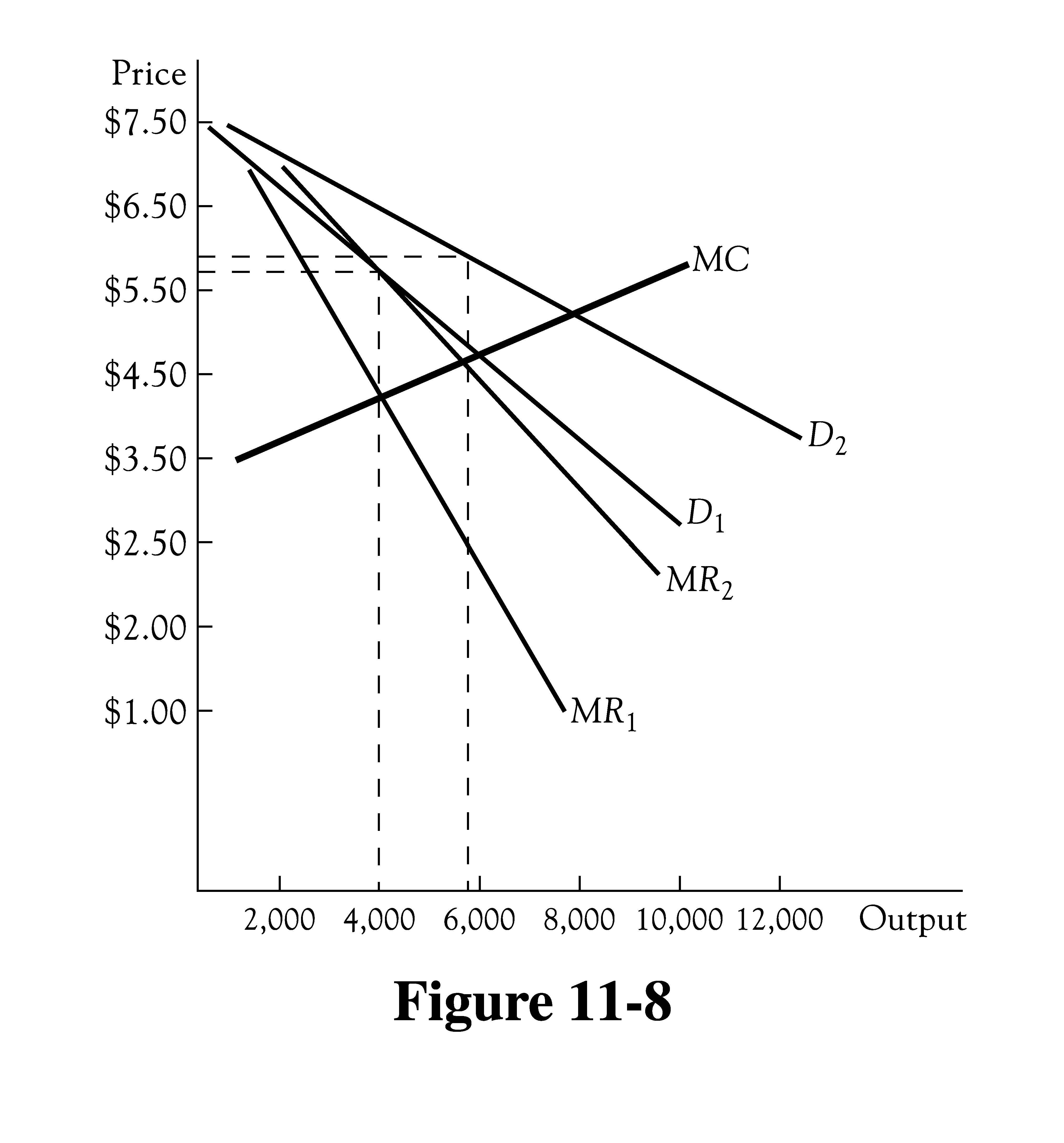
d. See Figure 11-8.
e. See Figure 11-8. The new output is between 5,700 and 5,800 units and price is between $5.90 and $6.00.
f. Nothing. The monopolist will continue to operate at this level of output and price until cost conditions change or there is another demand change or it changes its scale of operation.
g. The industry would return to the competitive level as entry would occur until zero profits were made by all firms.
4. a. P = MC/(1 - (1/)) = $1.00/0.5 = $2.00
b. Lerner index equals (P - MC)/P = ($2.00 - $1.00)/$1.00 = 0.5. (Note that this is equal to 1/).
5. A supply curve relates price and quantity supplied. Under monopoly, the profit-maximizing level of output is found by the rule MR = MC. Then price is found from the demand curve. Since many demand curves can be associated with MR = MC at a particular level of output, many prices can be associated with the level of output. That is, the price also depends on the demand curve.
6. Disagree. If the demand curve is linear, a higher price is associated with a more elastic demand. Hence an elastic demand may indicate that the monopoly is charging a high price. Further, we know a monopoly always produces on the elastic portion of its demand curve.
7. The monopolist may raise price if its costs increase, if demand increases, or both. The firm wants to maximize profits and not maximize revenues.
8. Agree. The determination of the market will be based on the availability of substitutes, which is also a key factor in determining whether the firm is a monopoly. A narrowing of the definition of the market means the number of goods that are accepted as close substitutes is reduced too, and this increases the likelihood that the firm will be considered a monopoly.
9. Yes, because iron ore is a key input in the production of steel. U.S. Steel is not a monopoly today because it no longer controls a key input. New iron ore discoveries around the world and increased foreign competition have caused U.S. Steel to lose its monopoly.
10. No. If the firm believes that new firms will enter at that price, but that a lower price would prevent entry and still allow the monopolist to earn some profits, it will charge a lower price.
11. A firm has monopoly power when it faces a demand curve that slopes down. Many firms that are not pure monopolies face downward-sloping demand curves, often because of product differentiation. Chapter 13 discusses those cases in more detail.
12. The source of the monopoly's bad effects is the downward-sloping demand curve, which implies that marginal revenue lies below price. This results in the monopolist's restricting output to the level for which MR = MC, which implies P > MC.
13. No. If there are substantial economies of scale, the costs of production for a monopolist may be lower than the costs if the industry was perfectly competitive. If so, it is possible for the monopoly to charge a lower price and produce more output.
14. Static analysis assumes that the existing goods and production processes are the only ones that matter, while dynamic analysis considers technological change and the introduction of new goods and services. Since society values new products, a firm that develops a new product still benefits society even if it charges a monopoly price. The alternative may be none of the good at all. Dynamic analysis suggests that antitrust policymakers should examine more than whether a firm currently is charging a monopoly price, but also look at how the firm obtained its position.
15. TR = PxQ but P = P(Q). Therefore, TR = P(Q)xQ and MR = P + (dP/dQ)Q. Under perfect competition, a firm has no control over price so dP/dQ = 0 and MR = P. If the firm is a monopoly it implies, dP/dQ < 0 so MR < P.
16. = TR - TC = 30Q -0.75Q2 - 20 - 9Q - .03Q2 (1)
To maximize profits, take derivative of (1) with respect to Q:
d/dQ = 30 - 1.5Q - 9 - 0.6Q = 0. (2)
Solving for Q yields the profit-maximizing level of output of 10 units.
Substituting 10 into (1) gives profits of $85.
Under perfect competition, P = MC:
30 - 0.75Q = 9 + 0.6Q; (3)
Solving for Q yields Q = 15.56 and P = 18.33.
244


