Hello , I need help with my excel assignment some part are wrong

Ballantyne Investments

IMPORT DATA AND INSERT SMARTART, IMAGES, AND CHARTS

GETTING STARTED

Open the file SC_EX19_7a_Mac_FirstLastName_1.xlsx, available for download from the SAM website.
Save the file as SC_EX19_7a_Mac_FirstLastName_2.xlsx by changing the “1” to a “2”.
If you do not see the .xlsx file extension in the Save As dialog box, do not type it. The program will add the file extension for you automatically.
To complete this SAM Project, you will also need to download and save the following data files from the SAM website onto your computer:
Support_EX19_7a_Mac_Disclaimer.pptx
Support_EX19_7a_Mac_Group.jpg
Support_EX19_7a_Mac_Sample.xlsx
Support_EX19_7a_Mac_Team.html
With the file SC_EX19_7a_Mac_FirstLastName_2.xlsx still open, ensure that your first and last name is displayed in cell B6 of the Documentation sheet.
If cell B6 does not display your name, delete the file and download a new copy from the SAM website.

PROJECT STEPS

Elena Dorado is an associate investment banker at Ballantyne Investments. She is preparing a draft of a workbook that will be presented to shareholders to describe Ballantyne's asset management team and client relationships. She asks for your help in importing data and adding other content to the workbook.
Go to the Asset Management worksheet. Change the formatting of cell D4 and the WordArt containing the worksheet title, "Ballantyne Investments", as follows to coordinate it with the rest of the worksheet:

1. Apply the Fill: Turquoise, Accent Color 1; Shadow WordArt Style to the title.
2. Copy the formatting from cell A4 to cell D4.

The worksheet should list information about the asset management team, which is contained in a webpage.
Copy data from the webpage as follows:

1. From the Data tab, use the 'From HTML' tool to open the webpage Support_EX19_7a_Mac_Team.html as a table in a new workbook.
2. Copy the table, with the column headers included, from the new worksheet. In the Asset Management worksheet, paste the table in cell G12. Close the new worksheet without saving.
3. Format the pasted data in the range G12:M19 as a table using Turquoise, Table Style Light 9. (Hint: Make sure "My table has headers" is checked.)

In the new table, change some data to reflect updates in the company:

1. Delete the row for Employee 520 because Chad Johnson is no longer with Ballantyne Investments.
2. Find the text "Financial advisor" and replace it with Investments to use a position name the company recently updated.

Elena wants to list the team information in the range A5:E10. The webpage table separated the first and last names, but Elena wants to list the full name on the Asset Management worksheet.
List the first and last names of each team member in a single cell as follows:

1. In cell A5, enter a formula using the CONCAT function that displays the first name shown in cell H13 followed by a space (" ") and then the last name shown in cell I13.
2. Fill the range A6:A10 with the formula in cell A5 to list the full names of the remaining team members.

Incorporate the imported data in the range B5:E10 as follows:

1. Copy the Position data from the range J13:J18 and paste only the values in the range B5:B10.
2. In cell C5, enter a formula using the PROPER function to capitalize the first letter in each word in the Specialty text in cell K13.
3. Fill the range C6:C10 with the formula in cell C5 to list the specialties of the remaining team members.
4. In cell D5, enter a formula using the LEFT function to insert the first 2 characters on the left of cell L13. Copy the formula in cell D5 to the range D6:D10.
5. In cell E5, enter a formula using the RIGHT function to insert the last 2 characters on the right of cell M13. Copy the formula in cell E5 to the range E6:E10.
6. Resize columns A:D to their best fit, resize columns E:F to 7.00, and size column G to 21.00.
7. Hide rows 12 to 18 so that the worksheet does not display duplicated data.

Elena already imported data summarizing the performance of the asset management team on the Performance Summary worksheet but wants to display the data in the range G5:H8 of the Asset Management worksheet. She asks you to switch the rows and columns when you insert the data to fit in the range G5:H8.
Go to the Performance Summary worksheet. Copy the data in the range A1:D2, and then transpose the rows and columns as you paste the data on the Asset Management worksheet starting in cell G5.
In the Asset Management worksheet, insert and format a picture of the asset management team as follows so that shareholders can identify members of the team:

1. Insert the picture Support_EX19_7a_Mac_Group.jpg.
2. Move and resize the picture proportionally so that the upper-left corner is in cell G19 and the lower-right corner is in cell J36.
3. Add a border to the picture using Teal, Accent 6 as the border color to coordinate the picture with the rest of the worksheet.
4. Apply the Offset: Center picture effect from the Outer section of the Shadow gallery.

Add a caption to identify the picture as follows:

1. In cell H37, insert a Text Box from the Basic Shapes section of the Shapes gallery.
2. Enter Asset management team at work in the text box.
3. Resize the text box to display the entire caption and move the text box so that it is centered below the picture in the range G37:J38.

Elena also wants to provide an organization chart to show the hierarchy of the asset management team.
Insert an organization chart as follows:

1. Insert the Organization Chart SmartArt from the Hierarchy section of the SmartArt gallery.
2. Move and resize the SmartArt so that the upper-left corner is in cell A19 and the lower-right corner is in cell D36.

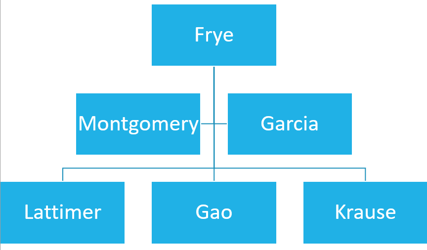
Add text to the SmartArt as follows, using Figure 1 as a guide:

1. Enter Frye in the top shape.
2. Enter Montgomery in the second shape.
3. Add a shape after the "Montgomery" shape so that it appears to the right of the "Montgomery" shape.
4. Enter Garcia in the new shape.
5. In the bottom row, enter Lattimer in the left shape.
6. Enter Gao in the middle shape.
7. Enter Krause in the right shape.

Figure 1: SmartArt Text

Hello , I need help with my excel assignment some part are wrong 1

Add a caption to identify the SmartArt as follows:

1. In cell B37, insert a Text Box from the Basic Shapes section of the Shapes gallery.
2. Enter Org chart in the text box.
3. Resize the text box to display the entire caption and align the top of the "Org chart" text box with the top of the "Asset management team at work" text box in row 37.

Hide the gridlines on the worksheet to increase its visual appeal.
Elena wants to include the company slogan and a standard disclaimer about Ballantyne Investments services on the Asset Management worksheet. She has this information stored in a PowerPoint presentation. Include the information as follows:

1. Use PowerPoint to open the presentation Support_EX19_7a_Mac_Disclaimer.pptx.
2. In Excel, use the Screen Clipping tool to paste a screenshot of only the slogan and disclaimer into the Asset Management worksheet.
3. Position the upper-left corner of the screenshot image in cell B40.

Go to the Client Investment Tracker worksheet, which Elena asks you to finish. The worksheet shows sample data for a fictional client to illustrate the type of information Ballantyne Investments provides to its clients.
Elena inserted the data in the range A20:C28 as a link to another worksheet. Complete the sample data and break the link as follows:

1. In cell B29, use the Sum function to insert the total investment amount from the range B21:B28, which should match the total in cell D28.
2. Create a conditional formatting rule using the Solid Fill Blue Data Bar option to the range F21:F28 to help clients visualize the data.
3. Break the link to the Support_EX19_7a_Mac_Sample.xlsx workbook because Elena no longer needs to update the date.

Elena wants to show the total amount invested compared to the total value during the eight months of investments.
Insert a chart in the Client Investment Tracker worksheet as follows to show this information:

1. Based on the nonadjacent data in the Date (range A20:A28), Total Value (range C20:C28), and Total Invested (range D20:D28) columns, insert the first type of chart that Excel recommends, which is a Clustered Column – Line chart.
2. Move and resize the chart so that its upper-left corner is in cell A5 and its lower-right corner is in cell F19.
3. Remove the chart title because the legend identifies the data clearly.

Elena wants to make sure that people reviewing the worksheet understand it displays sample data.
Add a shape to the worksheet as follows to provide this information:

1. In cell E30, insert a Line Callout 1 shape from the Callouts section of the Shapes gallery.
2. Move the callout line so that it points to the bottom of the "Total Invested" column.
3. Type Sample data only in the callout shape.
4. Apply the Subtle Effect – Turquoise, Accent 1 shape style to the callout shape.

Elena wants to format the column chart in the range G20:M33 to call attention to it. She also wants to change the layout of the chart so that it provides another way to compare the total amounts by month.
Modify the column chart as follows:

1. Switch the rows and columns so that the chart compares the total value and the total invested by months 1 to 8.
2. Apply the Ice Blue, Background 2 shape fill color to the plot area of the chart.
3. Apply the Offset: Bottom Right shape effect from the Outer section of the Shadow gallery to the legend.

Elena wants to add one more element of visual interest on the worksheet.

1. Insert an online picture using investments as the search text. Select the first picture in the search results. Delete the textbox underneath with the attribution.
2. Reposition and resize the picture so that the upper-left corner is in cell G1 and the bottom-right corner is in cell K13.

Your workbook should look like the Final Figures on the following pages. Save your changes, close the workbook, and then exit Excel. Follow the directions on the SAM website to submit your completed project.

Final Figure 1: Asset Management Worksheet

Hello , I need help with my excel assignment some part are wrong 2

Final Figure 2: Client Investment Tracker Worksheet

Hello , I need help with my excel assignment some part are wrong 3