ALL THE QUESTIONS ARE IN THE FILE ATTACHED

1 True or false questions. 10 points

Mark the correct answer

1. Under the assumption of conditional mean independence, it is possible to state that the OLS estimator for the parameter of interest is unbiased (True / False)

2. Under simple random sampling, the observations in a sample are not identically independently distributed. (True / False)

3. It is possible to calculate the OLS estimator under perfect multicollinearity. (True/False)

4. The sample mean is an unbiased estimator of the expected value of the population parameter (True/False)

5. It is always possible to show that an estimator is unbiased, regardless of the particular form of its formula (True/False)

6. An unbiassed estimator produces, on average, the true value of the parameter for which it was constructed. (True/False).

2 Theoretical questions. 40 points

I. Answer the following questions in your own words. Extra points will be granted for including formal derivations in the questions that do not explicitly require them.

1. Define what is a false positive and a false negative in the context of hypothesis testing.

2. Explain in a detailed manner and denoting each step in the process, how to evaluate the statistical significance of the value taken by an estimator

3. Show why if E[u|x] not equal to 0 , then the OLS estimator is not unbiassed

4. Show why calculating the simple difference in means between two groups of observations may fail to produce an estimation of the causal effect. Explain the type of bias that could happen in this context.

3 Application questions. 50 points

Read carefully the following and answer all the questions. The information is provided in the table below. State all the relevant formulas and all your calculations.

You are part of a World Bank mission to the country of Tatooine created with the objective of evaluating two policy policy programs in terms of their effect on household income per person. The first one is an agricultural training program targeted to the population that is concentrated in the most fertile region of the country. The second program is a subsidy designed to incentivize engagement in activities related machinery production and repair among the population that lives in the infertile regions of the country. It is known that educational attainment levels, family composition and other sociodemographic variables vary according to the region inhabited. That is, the sociodemographic variables are different between the most fertile and the most infertile regions.

Due to budgetary constraints, none of the programs was able to cover its target population in full. Taking advantage of this limitation, the policy makers decided to randomize the assignment of the programs across its target populations.

The first program was designed as follows. Those that were selected into the treatment group received a semester long training program on how to take advantage of the characteristics of the land they owned. That is, they were introduced to the type of crops that have the highest yields and that can be produced in the region, the different production processes that can be implemented due to the geological characteristics and so on. The population that is part of the control group did not received any training.

The second program consisted on a fixed subsidy to the employers in the manufacturing and repair service sector per local worker employed. This means that on a monthly basis, employers told the government how many local employees they have in the payroll, the government verified the information, and transferred an amount kL to the employer, where k is the subsidy amount, and L the number of local employees hired.

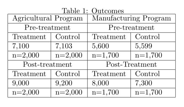
Both programs have been instrumented over the last two years. Table 1) shows the average household income of the control and treatment group of each intervention both at the moment the programs were started, and at the moment you arrived to evaluate them. The table also shows the size of each group.

Table 1:

• What condition, or conditions, need to hold in order for the randomization to have been correctly implemented?.

• Assume that condition, or conditions, hold. Your task is to evaluate if, at the end of the day, the program had an effect on the household income per capita of the treated population with respect to those in the control group. Calculate the ATE of each program on the final level of household income per capita, assuming that all the individuals are compliers.

• Evaluate if the effect is statistically different from zero at the usual confidence levels. For this case, the standard errors have to be calculated following the formula:

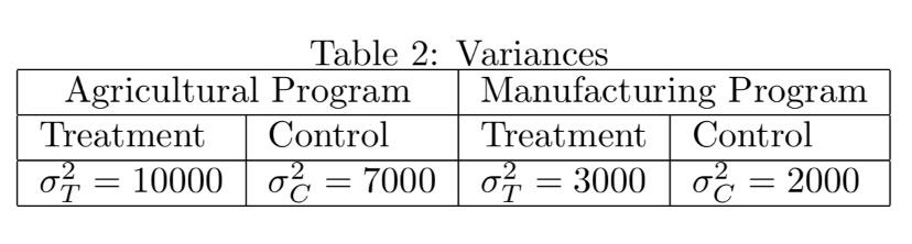
where nT corresponds to the sample size of the treated group, nC to the sample size of the control group, σ 2 T , and σ 2 C are the variances of the treatment and the control group. The values for them are given in table 2. Remember that the critical values in the t distribution are the following: For 90% of confidence the value is 1.646, for 95% of confidence the value is 1.960, for 99% of confidence the value is 2.576 and 99.9% of confidence the value is 3.291.

Table 2:

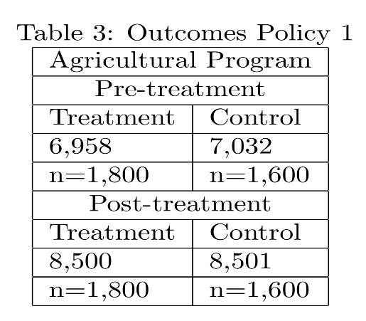
Later on, you get knowledge of the fact that some of the individuals who were assigned to receive the training program did not attend the training sessions, and instead, some individuals who were in the control group, show-up. Specifically, assume that 20% of those assigned the treatment did not showed up, and that 10% of those assigned to the control group received the treatment. Assume that the remaining percentages of each group are compliers who were affected by the randomization. You make the necessary adjustments and recalculate the average household income per capita of the treatment and control groups of the first policy intervention. The new information is presented in table 3

• Explain what is the Local Average Treatment Effect and how it is different from the ATE

• Calculate the LATE on the growth rates of the average household income

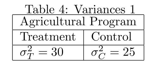
• Is that LATE statistically significant? Use the formula expressed previously to calculate the standard errors. The information on the variances of the growth rate information that you need in this case, is presented in table 4

Table 4: