Phase3 decision table and decision tree
8.4 LOGIC MODELING USING DECISION TABLES
Structured English can be used to represent the logic contained in an information system process, but sometimes a process's logic can become quite complex. If several different conditions are involved, and combinations of these conditions dictate which of several actions should be taken, then Structured English may not be adequate for representing the logic behind such a complicated choice. It is not that Structured English cannot represent complicated logic; rather, Structured English becomes more difficult to understand and verify as logic becomes more complicated. Research has shown, for example, that people become confused in trying to interpret more than three nested IF statements. When the logic is complicated, a diagram may be much clearer than a Structured English statement. A decision table is a diagram of process logic where the logic is reasonably complicated. All of the possible choices and the conditions the choices depend on are represented in tabular form, as illustrated in the decision table in Figure 8.5.
 Open table as spreadsheet
|
| Conditions/Courses of Action | Rules | |||||
| 1 | 2 | 3 | 4 | 5 | 6 | ||
| Condition Stubs | Employee type | S | H | S | H | S | H |
| Hours worked | <30 | <30 | 30 | 30 | >30 | >30 | |
|
|
|
|
|
|
|
| |
| Action Stubs | Pay base salary | x |
| x |
| x |
|
| Calculate hourly wage |
| x |
| x |
| x | |
| Calculate overtime |
|
|
|
|
| x | |
| Produce Absence Report |
| x |
|
|
|
| |
Fig. 8.5: Complete decision table for payroll system example
The decision table in Figure 8.5 models the logic of a generic payroll system. The table has three parts: the condition stubs, the action stubs, and the rules. The condition stubs contain the various conditions that apply to the situation the table is modeling. In Figure 8.5, there are two condition stubs for employee type and hours worked. Employee type has two values: "S," which stands for salaried, and "H," which stands for hourly. Hours worked has three values: less than 30, exactly 30, and more than 30. The action stubs contain all the possible courses of action that result from combining values of the condition stubs. There are four possible courses of action in this table: Pay Base Salary, Calculate Hourly Wage, Calculate Overtime, and Produce Absence Report. You can see that not all actions are triggered by all combinations of conditions. Instead, specific combinations trigger specific actions. The part of the table that links conditions to actions is the section that contains the rules.
To read the rules, start by reading the values of the conditions as specified in the first column: Employee type is "S," or salaried, and hours worked is less than 30. When both of these conditions occur, the payroll system is to pay the base salary. In the next column, the values are "H" and "<30," meaning an hourly worker who worked less than 30 hours. In such a situation, the payroll system calculates the hourly wage and makes an entry in the Absence Report Rule 3 addresses the situation when a salaried employee works exactly 30 hours. The system pays the base salary, as was the case for rule 1. For an hourly worker who has worked exactly 30 hours, rule 4 calculates the hourly wage. Rule 5 pays the base salary for salaried employees who work more than 30 hours. Rule 5 has the same action as rules 1 and 3 and governs behaviour with regard to salaried employees. The number of hours worked does not affect the outcome for rules 1,3, or 5. For these rules, hours worked is an indifferent condition in that its value does not affect the action taken. Rule 6 calculates hourly pay and overtime for an hourly worker who has worked more than 30 hours.
Because of the indifferent condition for rules 1, 3, and 5, we can reduce the number of rules by condensing rules 1, 3, and 5 into one rule, as shown in Figure 8.6. The indifferent condition is represented with a dash. Whereas we started with a decision table with six rules, we now have a simpler table that conveys the same information with only four rules.
Open table as spreadsheet
| Conditions/Courses of Action | Rules | |||
| 1 | 2 | 3 | 4 | |
| Employee type | ||||
| Hours worked | − | <30 | 30 | >30 |
| Pay base salary |
|
|
| |
| Calculate hourly wage |
| |||
| Calculate overtime |
|
|
| |
| Produce absence Report |
|
|
| |
Fig. 8.6: Reduced decision table for payroll system example
In constructing these decision tables, we have actually followed a set of basic procedures:
Name the conditions and the values that each condition can assume. Determine all of the conditions that are relevant to your problem and then determine all of the values each condition can take. For some conditions, the values will be simply "yes" or "no" (known as a limited entry). For others, such as the conditions in Figures 8.5 and 8.6, the conditions may have more values (known as an extended entry).
Name all possible actions that can occur. The purpose of creating decision tables is to determine the proper course of action given a particular set of conditions.
List all possible rules. When you first create a decision table, you have to create an exhaustive set of rules. Every possible combination of conditions must be represented. It may turn out that some of the resulting rules are redundant or make no sense, but these determinations should be made only after you have listed every rule so that no possibility is overlooked. To determine the number of rules, multiply the number of values for each condition by the number of values for every other condition. In Figure 8.5, we have two conditions, one with two values and one with three, so we need 2 × 3, or 6 rules. If we added a third condition with four values, we would need 2 × 3 × 4, or 24 rules.
When creating the table, alternate the values for the first condition, as we did in Figure 8.5 for type of employee. For the second condition, alternate the values but repeat the first value for all values of the first condition, then repeat the second value for all values of the first condition, and so on. You essentially follow this procedure for all subsequent conditions. Notice how we alternated the values of hours worked in Figure 8.5. We repeated "<30" for both values of type of employee, "S" and "H." Then we repeated "30," and then ">30"
Define the actions for each rule. Now that all possible rules have been identified, provide an action for each rule. In our example, we were able to figure out what each action should be and whether all of the actions made sense. If an action doesn't make sense, you may want to create an "impossible" row in the action stubs in the table to keep track of impossible actions. If you can't tell what the system ought to do in that situation, place question marks in the action stub spaces for that particular rule.
Simplify the decision table. Make the decision table as simple as possible by removing any rules with impossible actions. Consult users on the rules where system actions aren't clear and either decide on an action or remove the rule. Look for patterns in the rules, especially for indifferent conditions. We were able to reduce the number of rules in the payroll example from six to four, but greater reductions are often possible.
A decision tree is a graphical technique that depicts a decision or choice situation as a connected series of nodes and branches. Decision trees were first devised as a management science technique to simplify a choice where some of the needed information is not known for certain. By relying on the probabilities of certain events, a management scientist can use a decision tree to choose the best course of action. Although this type of decision tree is beyond the scope of our text, we can use modified decision trees (without the probabilities) to diagram the same sorts of situations for which we used decision tables. Why introduce yet another diagramming technique to do what a decision table does? Both decision tables and decision trees are communication tools designed to make it easier for analysts to communicate with users. Deciding exactly which technique to use depends on various factors, which we discuss in detail in the next section, after you have an understanding of decision trees.
As used in requirements structuring, decision trees have two main components: decision points, which are represented by nodes, and actions, which are represented by ovals. Figure 8.7 shows a generic decision tree. To read a decision tree, you begin at the root node on the far left. Each node is numbered, and each number corresponds to a choice; the choices are spelled out in a legend for the diagram. Each path leaving a node corresponds to one of the options for that choice. From each node, there are at least two paths that lead to the next step, which is either another decision point or an action. Finally, all possible actions are listed on the far right of the diagram in leaf nodes. Each rule is represented by tracing a series of paths from the root node, down a path to the next node, and so on, until an action oval is reached.
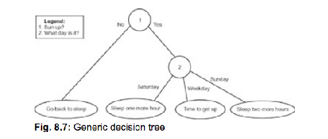
Fig. 8.7: Generic decision tree
Look back at the decision tables we created for the payroll system logic (Figures 8.5 and 8.6). There are at least two ways to represent this same information as a decision tree. The first is shown in Figure 8.8. Here, all of the choices are limited to two outcomes, either yes or no. However, looking at how the conditions are phrased in the decision tables, you remember that hours worked has three values, not two. You might argue that forcing a condition with three values into a set of conditions that has only yes or no available as values is somewhat artificial.
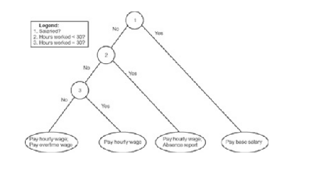
Fig. 8.8: Decision tree representation of the decision logic in decision tables shown in figures 8.5 and 8.6, with only two choices per decision point
To preserve the original logic of the decision situation, you can draw your decision tree as depicted in Figure 8.9. Here, there are only two conditions; the first condition has two values and the second has three values, as is true in the decision table.
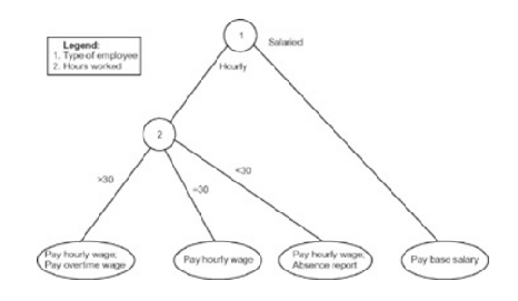
Fig. 8.9: Decision tree representation of the decision logic in the decision tables shown in figures 8.5 and 8.6, with multiple choices per decision point
We have waited until now to make two important points about decision tables and decision trees. Once you have spent some time creating logic modeling aids such as these, be ready to refine them by drawing the diagrams again and again. As was the case with data flow diagrams, decision tables and decision trees benefit greatly from iteration. The second point is that you should always share your work with other team members and users to get feedback on the mechanical and content accuracy of your work. Other team members and users will often provide insight into issues you might have overlooked in describing the logic. For that reason, it is not uncommon for the analysis team leader to schedule a walkthrough at some point during the requirements structuring process.


