Problem Set Week Two
Lecture 4
(Sampling basics and Hypothesis test)
This week we turn from descriptive statistics to inferential statistics and making decisions
about our populations based on the samples we have. For example, our class case research
question is really asking if in the entire company population of employees, do males and females
receive the same pay for doing equal work. However, we are not analyzing the entire
population, instead we have a sample of 25 males and 25 females to work with.
This brings us to the idea of sampling – taking a small group/sample from a larger
population. To paraphrase, not all samples are created equal. For example, if you wanted to
study religious feelings in the United States, would you only sample those leaving a
fundamentalist church on a Wednesday? While this is a legitimate element of US religions, it
does not represent the entire range of religious views – it is representative of only a portion of the
US population, and not the entire population.
The key to ensuring that sample descriptive statistics can be used as inferential statistics –
sample results that can be used to infer the characteristics (AKA parameters) of a population – is
have a random sample of the entire population. A random sample is one where, at the start,
everyone in the population has the same chance of being selected. There are numerous ways to
design a random sampling process, but these are more of a research class concern than a
statistical class issue. For now, we just need to make certain that the samples we use are
randomly selected rather than selected with an intent of ensuring desired outcomes are achieved.
The issue about using samples that students often new to statistics is that the sample
statistic values/outcomes will rarely be exactly the same as the population parameters we are
trying to estimate. We will have, for each sample, some sampling error, the difference between
the actual and the sample result. Researchers feel that this sampling error is generally small
enough to use the data to make decisions about the population (Lind, Marchel, & Wathen,
2008).
While we cannot tell for any given sample exactly what this difference is, we can
estimate the maximum amount of the error. Later, we will look at doing this; for now, we just
need to know that this error is incorporated into the statistical test outcomes that we will be
studying.
Once we have our random sample (and we will assume that our class equal pay case
sample was selected randomly), we can start with our analysis. After developing the descriptive
statistics, we start to ask questions about them. In examining a data set, we need to not only
identify if important differences exist or not but also to identify reasons differences might exist.
For our equal pay question, it would be legal to pay males and females different salaries if, for
example, one gender performed the duties better, or had more required education, or have more
seniority, etc. Equal pay for equal work, as we are beginning to see, is more complex than a
simple single question about salary equality. As we go thru the class, we will be able to answer
increasingly more complex questions. For this week, we will stay with questions about
involving ways to sort our salary results – looking for differences might exist.
Some of these questions for this week with our equal pay case could include:
• Could the means for both males and females be the same, and the observed difference
be due to sampling error only?
• Could the variances for the males and female be the same (AKA statistically equal)?
• Could salaries per grade be statistically equal?
• Could salaries per degree (undergraduate and graduate) be the same?
• Etc.
Hypothesis Testing
As we might expect, research and statistics have a set procedure/process on how to go
about answering these questions. The hypothesis testing procedure is designed to ensure that
data is analyzed in a consistent and recognized fashion so everyone can accept the outcome.
Statistical tests focus on differences – is this difference large enough to be significant,
that is not simply a sampling error? If so, we say the difference is statistically significant; if not,
the difference is not considered statistically significant. This phrasing is important as it is easy to
measure a difference from some point, it is much harder to measure “things are different.” It is
that pesky sampling error that interferes with assessing differences directly.
Before starting the hypothesis test, we need to have a clear research question. The
questions above are good examples, as each clearly asks if some comparison is statistically equal
or not. Once we have a clear question – and a randomly drawn sample – we can start the
hypothesis testing procedure. The procedure itself has five steps:
• Step 1: State the null and alternate hypothesis
• Step 2: Form the decision rule
• Step 3: Select the appropriate statistical test
• Step 4: Perform the analysis
• Step 5: Make the decision, and translate the outcome into an answer to the initial
research question.
Step 1. The null hypothesis is the “testable” claim about the relationship between the
variables. It always makes the claim of no difference exists in the populations. For the question
of male and female salary equality, it would be: Ho: Male mean salary = Female mean salary.
If this claim is found not to be correct, then we would accept the alternate hypothesis claim: Ha:
Male salary mean =/= (not equal) Female salary mean. (Note, some alternate ways of phrasing
these exist, and we will cover them shortly. For now, let’s just go with this format.)
Step 2. This step involves selecting the decision rule for rejecting the null hypothesis
claim. This will be constant for our class – we will reject the null hypothesis when the p-value is
equal to or less than 0.05 (this probability is called alpha). Other common values are .1, and .01
– the more severe the consequences of being wrong if we reject the null, the smaller the value of
alpha we select. Recall that we defined the p-value last week as the probability of exceeding a
value, the value in this case would be the statistical outcome from our test.
Step 3. Selecting the appropriate statistical test is the next step. We start with a question
about mean equality, so we will be using the T-test – the most appropriate test to determine if
two population means are equal based upon sample results.
Step 4. Performing the analysis comes next. Fortunately for us, we can do all the
arithmetic involved with Excel. We will go over how to select and run the appropriate T-test
below.
Step 5. Interpret the test results, making a decision on rejecting or not rejecting the null
hypothesis, and using this outcome to answer the research question is the final step. Excel output
tables provide all the information we need to make our decision in this step.
Step 1: Setting up the hypothesis statements
In setting up a hypothesis test for looking at the male and female means, there are
actually three questions we could ask and associated hypothesis statements in step 1.
1. Are male and female mean salaries equal?
a. Ho: Male mean salary = Female mean salary
b. Ha: Male mean salary =/= Female mean salary
2. Is the male mean salary equal to or greater than the Female mean salary?
a. Ho: Male mean salary => Female mean salary
b. Ha: Male mean salary < Female mean salary
3. Is the male salary equal to or less than the female mean salary?
a. Ho: Male mean salary <= Female mean salary
b. Ha: Male mean salary > Female mean salary
While they appear similar each answers a different question. We cannot, for example,
take the first question, determine the means are not equal and then say that, for example, the
male mean is greater than the female mean because the sample results show this. Our statistical
test did not test for this condition. If we are interested in a directional difference, we need to use
a directional set of hypothesis statements as shown in statements 2 and 3 above.
Rules. There are several rules or guidelines in developing the hypothesis statements for
any statistical test.
1. The variables must be listed in the same order in both claims.
2. The null hypothesis must always contain the equal (=) sign.
3. The null can contain an equal (=), equal to or less than (<=) or equal to or greater than
(=>) claim.
4. The null and alternate hypothesis statement must, between them, account for all
possible actual comparisons outcomes. So, if the null has the equal (=) claim, the
alternate must contain the not equal (=/= or ≠) statement. If the null has the equal or
less than (<= or ≤) claim, the alternate must contain the greater than (>) claim.
Finally, if the null has the equal to or greater (=> or ≥) claim, the null must contain
the less than (<) claim.
Deciding which pair of statements to use depends on the research question being asked –
which is why we always start with the question. Look at the research question being asked; does
it contain words indicating a simple equality (means are equal, the same, etc.) or inequality (not
equal, different, etc.), if so we have the first example Ho: variable 1 mean = variable 2 mean, Ha:
variable 1 mean =/= variable 2 mean.
If the research question implies a directional difference (larger, greater, exceeds,
increased, etc. or smaller, less than, reduced, etc.) then it is often easier to use the question to
frame the alternate hypothesis and back into the null. For example, the question is the male
mean salary greater than the female mean salary would lead to an alternate of exactly what was
said (Ha: Male salary mean > Female salary mean) and the opposite null (Male salary mean <=
Female salary mean).
Step 2: Decision Rule
Once we have our hypothesis statements, we move on to deciding the level of evidence
that will cause us to reject the null hypothesis. Note, we always test the null hypothesis, since
that is where our claim of equality lies. And, our decision is either reject the null or fail to reject
the null. If the latter, we are saying that the alternate hypothesis statement is the more accurate
description of the relationship between the two variable population means. We never accept the
alternate.
When we perform a statistical test; we are in essence asking if, based on the evidence we
have is, the difference we observe be large enough to have been caused by something other than
chance or is it due to sampling error?
A statistical test gives us a statistic as a result. We know the shape of the statistical
distribution for each type of test, therefore we can easily find the probability of exceeding this
test value. Remember we called this the p-value.
Now all we need to decide is what is an acceptable level of chance – that is, when would
the outcome be so rare that we would not expect to see it purely by chance sampling error alone?
Most researchers agree that if the p-value is 5% (.05) or less than, then chance is not the cause of
the observed difference, something else must be responsible. This decision point is called alpha.
Other values of alpha frequently used are 10% (often used in marketing tests) and 1% (frequently
used in medical studies). The smaller the chosen alpha is, the more serious the error is in
rejecting the null when we should not have.
For our analysis, we will use an alpha of .05 for all our tests.
Final Point
You may have noticed that we have two basic types of hypothesis statements – those
testing equality and those testing directional differences. This leads to two different types of
statistical tests – the two-tail and the one-tail. In the one-tail test, the entire value of alpha is
focused on the distribution tail – either the right or left tail depending upon the phrasing of the
alternate hypothesis. A neat hint, the arrow head in the alternate hypothesis shows which tail the
result needs to be in to reject the null.
In the case of the two-tail test (equality), we do not care if one variable is bigger or
smaller than the other, only that they differ. This means that the rejection statistic could be in
either tail, the right or left. Since the reject region is split into two areas, we need to split alpha
into these areas – so with a two-tail test, we use alpha/2 as the comparison with our p-value (e.g.,
0.05/2 = 0.025). The example in Lecture 5 will review this in more detail.
References
Lind, D. A., Marchel, W. G., & Wathen, S. A. (2008). Statistical Techniques in Business &
Finance. (13th Ed.) Boston: McGraw-Hill Irwin.
Lecture 5
The T-Test
In the previous lecture, we introduced the hypothesis testing procedure, and developed
the first two steps of a statistical test to determine if male and female mean salaries could be
equal in the population – where our differences were caused simply by sampling errors. This
lecture continues with this example by completing the final three steps. It also introduces our
first statistical test, the t-test for mean equality.
Last week we looked at the normal curve and noted several of its characteristics, such as
mean = median = mode, symmetrical around the mean, curve height drops off the further the
score gets from the mean (meaning scores further from the mean are less likely to occur). Our
first statistical test, the t-test, is based on a population that is distributed normally. The t-test is
used when we do not have the population variance value – this is the situation every time we use
a sample to make decisions about their related populations.
While the t-test has several different versions, we will focus on the most commonly used
form – the two sample test for mean equality assuming equal variance. When we are testing
measures for mean equality, it is fairly rare for the variances to be much difference, and the
observed difference is often merely sample error. (In Lecture 6, we will revisit this assumption.)
The logic of the test is that the difference between mean values divided by a measure of
this difference’s variation will provide a t statistic that is distributed normally, with the mean
equaling 0 and the standard deviation equaling 1. This outcome can then be tested to see what
the likelihood is that we would get a value this large or larger purely by chance – our old friend
the p-value. If this p-value exceeds our decision criteria, alpha, then we reject the null
hypothesis claim of no difference (Lind, Marchel, & Wathen, 2008).
Setting up the t-test
Before selecting any test from Excel, the data needs to be set up. For the t-test, there are
a couple of steps needed. First, copy the data you want to first set up the data. In our question
about male and female salaries, copy the gender variable column from the data page to a new
worksheet page (the recommendation is on the week 2 tab) and paste it to the right of the
questions (such as in column T), then copy and paste the salary values and paste them next to the
gender data. Next, sort both columns by the gender column – this will give you the salary data
sorted by gender. Then, in column V place the label/word Males, and in column W place the
label Females. Now copy the male salaries and paste them under the Male label, and do the
same for the female salaries and the female label. The data is now set up for easy entry into the
T-test data entry section.
The t-test is found in the Analysis Toolpak that was loaded into your Excel program last
week. To find it, click on the Data button in the top ribbon, then on the Data Analysis link in the
Analyze box at the right, then scroll down to the T-test: Two-Sample Assuming Equal Variances.
For assistance in setting up the t-test, please see the discussion in the Week 2 Excel Help lecture.
Interpreting the T-test Output
The t-test output contains a lot of information, and not all of it is needed to interpret the
result. The important elements of the t-test outcome will be shown with an example for our
research case question.
Equal Pay Example - continued
In Lecture 4 we set up the first couple of steps for our testing of the research question: Do
males and females receive equal pay for equal work? Our first examination of the data we have
for answering this question involves determining if the average salaries are the same.
Here is the completed hypothesis test for the question: Is the male average salary equal to
the female average salary?
Step 1. Ho: Male mean salary = female mean salary
Ha: Male mean salary ≠ female mean salary
Step 2. Reject the null if the p-value is < (less than) alpha = .05.
Step 3. The selected test is the Two-Sample T-test assuming equal variances.
Step 4. The test results are below. The screen shot shows output table.
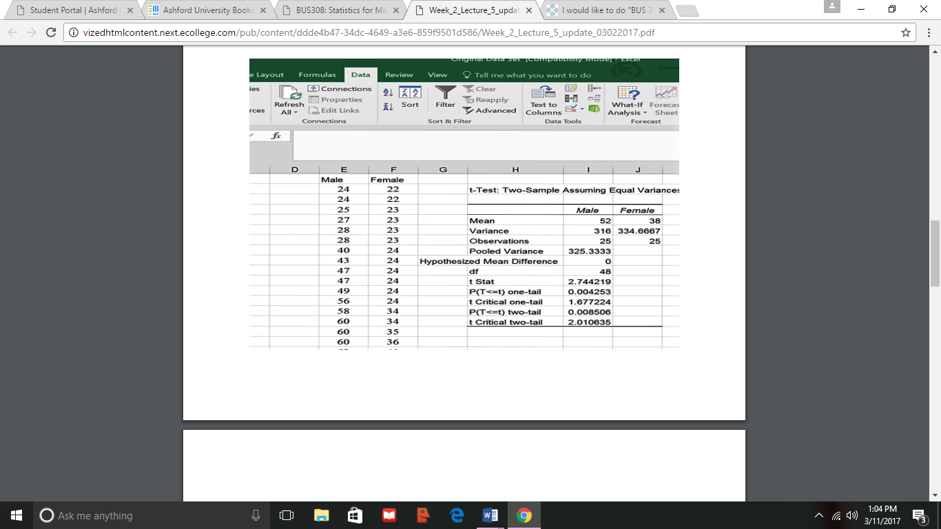
Step 5. Interpretation and conclusions.
The first step is to ensure we have all of the correct data. We see that we have 25 males
and females in the Observations row, and that the respective means are equal to what we earlier
calculated.
The calculated t statistic is 2.74 (rounded). We have two ways to determine if our result
rejects or fails to reject the null hypothesis; both involve the two-tail rows, as we have a two tail
test (equal or not equal hypothesis statements). The first is a comparison of the t-values – if the
critical t of 2.74 (rounded) is greater than the T-Critical two-tail value of 2.01, we reject the null
hypothesis. The second way is to compare the p-value with our criteria of alpha = .05.
Remember, since this is a two-tail test, the alpha for each tail is half of the overall alpha or .025.
If the p-value (shown as P(T<=t) two -tail value of 0.0085 is less than our one tail alpha (.025)
then we reject the null hypothesis. Note: at times Excel will report the p-value in an E format,
such as 3.45E-04. This is called an Exponent format, and is the same as 3.45 * 10-04. This
means move the decimal point 4 places to the left, making 3.45E-04 = 0.000345. Virtually any
p-value reported with an E-xx form will be less than our alpha of 0.05 (which would be 5E-02).
Since we rejected the null hypothesis in both approaches (and both will always provide
the same outcome), we can answer our question with: No - the male and female mean salaries are
not equal.
Note that for this set of data, we would have rejected the null for a one-tail test if and
only if the null hypothesis had been: Male mean salary is <= Female mean salary and the
alternate was Male mean salary is > Female mean salary. The arrow in the alternate points to the
positive/right tail and that is where the calculated t-statistic is. So, even if the p-value is smaller
than alpha in a one tail test, we need to ensure the t-statistic is in the correct tail for rejection.
References
Lind, D. A., Marchel, W. G., & Wathen, S. A. (2008). Statistical Techniques in Business &
Finance. (13th Ed.) Boston: McGraw-Hill Irwin.
Lecture 6
(Additional information on t-tests and hypothesis testing)
Lecture 5 focused on perhaps the most common of the t-tests, the two sample assuming
equal variance. There are other versions as well; Excel lists two others, the two sample assuming
unequal variance and the paired t-test. We will end with some comments about rejecting the null
hypothesis.
Choosing between the t-test options
As the names imply each of the three forms of the t-test deal with different types of data
sets. The simplest distinction is between the equal and unequal variance tests. Both require that
the data be at least interval in nature, come from a normally distributed population, and be
independent of each other – that is, collected from different subjects.
The F-test for variance.
To determine if the population variances of two groups are statistically equal – in order to
correctly choose the equal variance version of the t-test – we use the F statistic, which is
calculated by dividing one variance by the other variance. If the outcome is less than 1.0, the
rejection region is in the left tail; if the value is greater than 1.0, the rejection region is in the
right tail. In either case, Excel provides the information we need.
To perform a hypothesis test for variance equality we use Excel’s F-Test Two-Sample for
Variances found in the Data Analysis section under the Data tab. The test set-up is very similar
to that of the t-test, entering data ranges, checking Labels box if they are included in the data
ranges, and identifying the start of the output range. The only unique element in this test is the
identification of our alpha level.
Since we are testing for equality of variances, we have a two sample test and the rejection
region is again in both tails. This means that our rejection region in each tail is 0.25. The F-test
identifies the p-value for the tail the result is in, but does not give us a one and two tail value,
only the one tail value. So, compare the calculated p-value against .025 to make the rejection
decision. If the p-value is greater than this, we fail to reject the null; if smaller, we reject the null
of equal variances.
Excel Example. To test for equality between the male and female salaries in the
population, we set up the following hypothesis test.
Research question: Are the male and female population variances for salary equal?
Step 1: Ho: Male salary variance = Female salary variance
Ha: Male salary variance ≠ Female salary variance
Step 2: Reject Ho if p-value is less than Alpha = 0.025 for one tail.
Step 3: Selected test is the F-test for variance
Step 4: Conduct the test
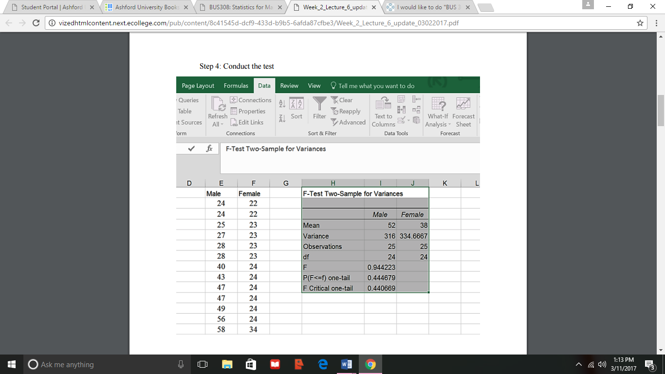
Step 5: Conclusion and interpretation. The test resulted in an F-value less than 1.0, so the
statistic is in the left tail. Had we put Females as the first variable we would have gotten a right
tail F-value greater than 1.0. This has no bearing on the decision. The F value is larger than the
critical F (which is the value for a 1-tail probability of 0.25 – as that was entered for the alpha
value).
So, since our p-value (.44 rounded) is > .025 and/or our F (0.94 rounded) is greater than
our F Critical, we fail to reject the null hypothesis of no differences in variance. The correct ttest
would be the two-sample T-test assuming equal variances.
Other T-tests.
We mentioned that Excel has three versions of the t-test. The equal and unequal variance
versions are set up in the same way and produce very similar output tables. The only difference
is that the equal variance version provides an estimate of the common variation called pooled
variance while this row is missing in the unequal variance version.
A third form of the t-test is the T-Test: Paired Two Sample for Means. A key
requirement for the other versions of the t-test is that the data are independent – that means the
data are collected on different groups. In the paired t-test, we generally collect two measures on
each subject. An example of paired data would be a pre- and post-test given to students in a
statistics class. Another example, using our class case study would the comparing the salary and
midpoint for each employee – both are measured in dollars and taken from each person. An
example of NON-pared data, would the grades of males and females at the end of a statistics
class. The paired t-test is set up in the same way as the other two versions. It provides the
correlation (a measure of how closely one variable changes when another does – to be covered
later in the class) coefficient as part of its output.
An Excel Trick. You may have noticed that all of the Excel t-tests are for two samples,
yet at times we might want to perform a one-sample test, for example quality control might want
to test a sample against a quality standard to see if things have changed or not. Excel does not
expressly allow this. BUT, we can do a one-sample test using Excel.
The reason is a bit technical, but boils down to the fact that the two-sample unequal
variance formula will reduce to the one-sample formula when one of the variables has a variance
equal to 0. So using the unequal variance t-test, we enter the variable we are interested – such as
salary – as variable one and the hypothesized value we are testing against – such as 45 for our
case – as variable two, ensuring that we have the same number of variables in each column.
Here is an example of this outcome.
Research question: Is the female population salary mean = 45?
Step 1: Ho: Female salary mean = 45
Ha: Female salary mean ≠ 45
Step 2: Reject the null hypothesis is less than Alpha = 0.05
Step 3: Selected test is the two sample unequal variance t-test
Step 4: Conduct the test
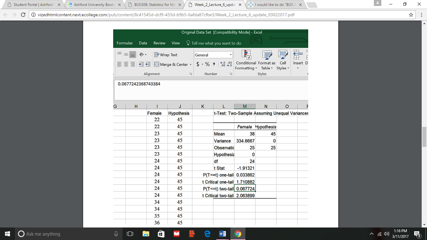
Step 5: Conclusions and Interpretation. Since the two tail p-value is greater than (>) .025
and/or the absolute value of the t-statistic is less than the critical two tail t value, we fail to reject
the null hypothesis. Our research question answer is that, based upon this sample, the overall
female salary average could equal 45.
Miscellaneous Issues on Hypothesis Testing
Errors. Statistical tests are based on probabilities, there is a possibility that we could
make the wrong decision in either rejecting or failing to reject the null hypothesis. Rejecting the
null hypothesis when it is true is called a Type I error. Accepting (failing to reject) the null when
it is false is called a Type II error.
Both errors are minimized somewhat by increasing the sample size we work with. A type
I error is generally considered the more severe of the two (imagine saying a new medicine works
when it does not), and is managed by the selection of our alpha value – the smaller the alpha, the
harder it is to reject the null hypothesis (or, put another way, the more evidence is needed to
convince us to reject the null). Managing the Type II error probability is slightly more
complicated and is dealt with in more advanced statistics class. Choosing an alpha of .05 for
most test situations has been found to provide a good balance between these two errors.
Reason for Rejection. While we are not spending time on the formulas behind our
statistical outcomes, there is one general issue with virtually all statistical tests. A larger sample
size makes it easier to reject the null hypothesis. What is a non-statistically significant outcome
based upon a sample size of 25, could very easily be found significant with a sample size of, for
example, 25,000. This is one reason to be cautious of very large sample studies – far from
meaning the results are better, it could mean the rejection of the null was due to the sample size
and not the variables that were being tested.
The effect size measure helps us investigate the cause of rejecting the null. The name is
somewhat misleading to those just learning about it; it does NOT mean the size of the difference
being tested. The significance of that difference is tested with our statistical test. What it does
measure is the effect the variables had on the rejection (that is, is the outcome practically
significant and one we should make decisions using) versus the impact of the sample size on the
rejection (meaning the result is not particularly meaningful in the real world).
For the two-sample t-test, either equal or unequal variance, the effect size is measured by
Cohen’s D. Unfortunately, Excel does not yet provide this calculation automatically, however it
is fairly easy to generate.
Cohen’s D = (absolute value of the difference between the means)/the standard deviation of both
samples combined.
Note: the total standard deviation is not given in the t-test outputs, and is not the same as the
square root of the pooled variance estimate. To get this value, use the fx function stdev.s on the
entire data set – both samples at the same time.
Interpreting the effect size outcome is fairly simple. Effect sizes are generally between 0
and 1. A large effect (a value around .8 or larger) means the variables and their interactions
caused the rejection of the null, and the result has a lot of practical significance for decision
making. A small effect (a value around .2 or less) means the sample size was more responsible
for the rejection decision than the variable outcomes. The medium effect (values around .5) are
harder to interpret and would suggest additional study (Tanner & Youssef-Morgan, 2013).
References
Lind, D. A., Marchel, W. G., & Wathen, S. A. (2008). Statistical Techniques in Business &
Finance. (13th Ed.) Boston: McGraw-Hill Irwin.
Tanner, D. E. & Youssef-Morgan, C. M. (2013). Statistics for Managers. San Deigeo, CA:
Bridgepoint Education.


