Assessment on One-Way ANOVA
![]()

Note: This guide is an example of creating ANOVA output in SPSS with the grades.sav file. The variables shown in this guide do not correspond with the actual variables assigned in Assessment 4. Carefully follow the instructions in the assignment for a list of assigned variables. Screen shots were created with SPSS 21.0.
Creating One-Way ANOVA OutputTo complete Section 2 of the DAA for Assessment 4, you will generate SPSS output for a histogram, descriptive statistics, and the Shapiro-Wilk test, which are covered in previous step-by-step guides. The Levene test (homogeneity of variance) is covered in the steps below.
Refer to the Assessment 4 instructions for a list of assigned variables. The example variables year and final are shown below.
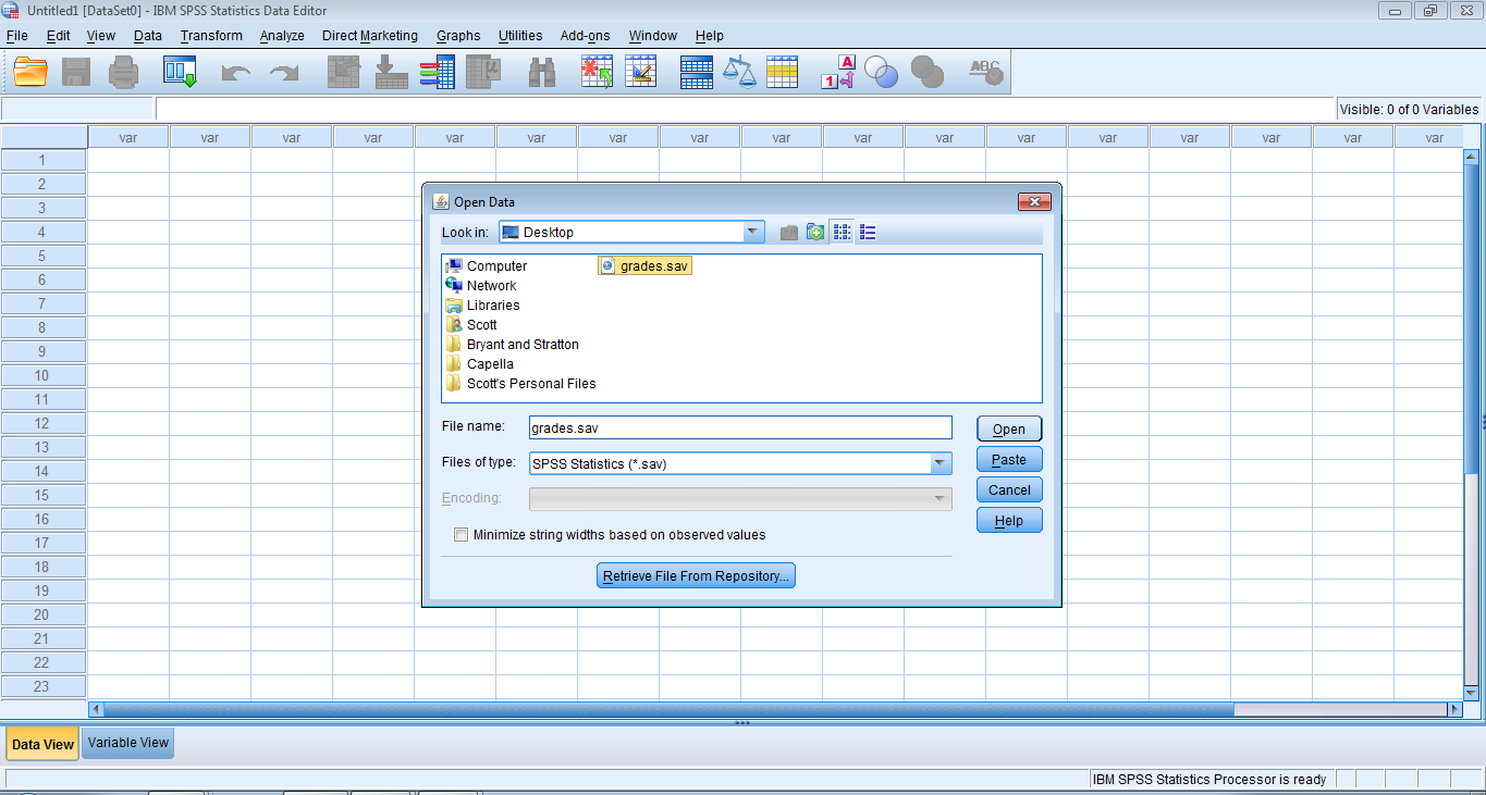
Step 1. Open grades.sav in SPSS.
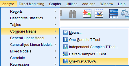
Step 2. On the Analyze menu, point to Compare Means and click One-Way ANOVA…
Step 3. In the One-Way ANOVA dialog box:
Move the assigned dependent variable into the Dependent List box.
Move the assigned independent variable into the Factor box. The examples of final and year are shown below.
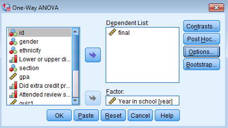
Click the Options button.
Step 4. In the One-Way ANOVA: Options dialog box:
Select Homogeneity of variance test (for the Levene test for Section 2 of the DAA).
Select Descriptive and Means Plot (for Section 4 of the DAA).
Click Continue.

Return to the One-Way ANOVA dialog box and select the Post Hoc button.
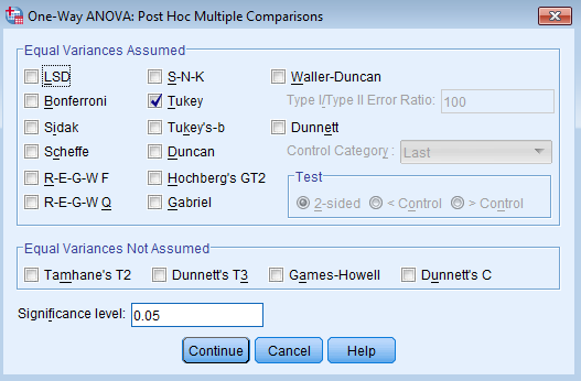
Step 5. In the One-Way ANOVA: Post Hoc Multiple Comparisons dialog box:
Check the Tukey option for multiple comparisons.
Click Continue and OK.
A string of ANOVA output will appear in SPSS. (The output below is for the example variable final.)
Step 1. Copy the Levene test output from SPSS and paste it into Section 2 of the DAA Template. Then interpret it for the homogeneity of variance assumption.
| Test of Homogeneity of Variances | |||
| final | |||
| Levene Statistic | df1 | df2 | Sig. |
| .866 | 3 | 101 | .462 |
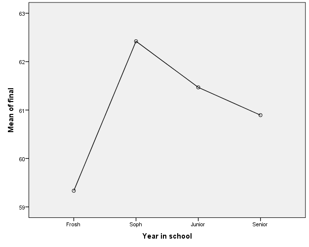
Step 2. Copy the means plot, paste it into Section 4 of the DAA Template, and interpret it.
Step 3. Copy the descriptives output. Paste it into Section 4 along with the report of means and standard deviations of the dependent variable at each level of the independent variable.
| Descriptives | ||||||||
| final | ||||||||
| N | Mean | Std. Deviation | Std. Error | 95% Confidence Interval for Mean | Minimum | Maximum | ||
| Lower Bound | Upper Bound | |||||||
| Frosh | 3 | 59.33 | 5.859 | 3.383 | 44.78 | 73.89 | 55 | 66 |
| Soph | 19 | 62.42 | 6.628 | 1.520 | 59.23 | 65.62 | 48 | 72 |
| Junior | 64 | 61.47 | 8.478 | 1.060 | 59.35 | 63.59 | 40 | 75 |
| Senior | 19 | 60.89 | 7.951 | 1.824 | 57.06 | 64.73 | 43 | 74 |
| Total | 105 | 61.48 | 7.943 | .775 | 59.94 | 63.01 | 40 | 75 |
Step 4. Copy the ANOVA output, paste it into Section 4, and interpret it.
| ANOVA | |||||
| final | |||||
| Sum of Squares | df | Mean Square | F | Sig. | |
| Between Groups | 37.165 | 3 | 12.388 | .192 | .902 |
| Within Groups | 6525.025 | 101 | 64.604 | ||
| Total | 6562.190 | 104 | |||
Step 5. Finally, if the overall ANOVA is significant, copy the post hoc output, paste it into Section 4, and interpret it.
| Multiple Comparisons | ||||||
| Dependent Variable: final | ||||||
| Tukey HSD | ||||||
| (I) Year in school | (J) Year in school | Mean Difference (I-J) | Std. Error | Sig. | 95% Confidence Interval | |
| Lower Bound | Upper Bound | |||||
| Frosh | Soph | -3.088 | 4.993 | .926 | -16.13 | 9.96 |
| Junior | -2.135 | 4.748 | .970 | -14.54 | 10.27 | |
| Senior | -1.561 | 4.993 | .989 | -14.61 | 11.48 | |
| Soph | Frosh | 3.088 | 4.993 | .926 | -9.96 | 16.13 |
| Junior | .952 | 2.100 | .969 | -4.53 | 6.44 | |
| Senior | 1.526 | 2.608 | .936 | -5.29 | 8.34 | |
| Junior | Frosh | 2.135 | 4.748 | .970 | -10.27 | 14.54 |
| Soph | -.952 | 2.100 | .969 | -6.44 | 4.53 | |
| Senior | .574 | 2.100 | .993 | -4.91 | 6.06 | |
| Senior | Frosh | 1.561 | 4.993 | .989 | -11.48 | 14.61 |
| Soph | -1.526 | 2.608 | .936 | -8.34 | 5.29 | |
| Junior | -.574 | 2.100 | .993 | -6.06 | 4.91 | |
6


