Assignment 2: Probability Analysis

SAMPLING MEAN:

DEFINITION:

The term sampling mean is a statistical term used to describe the properties of statistical distributions. In statistical terms, the sample mean from a group of observations is an estimate of the population mean. Given a sample of size n, consider n independent random variables X1, X2... Xn, each corresponding to one randomly selected observation. Each of these variables has the distribution of the population, with mean and standard deviation. The sample mean is defined to be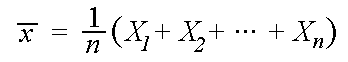

WHAT IT IS USED FOR:

It is also used to measure central tendency of the numbers in a database. It can also be said that it is nothing more than a balance point between the number and the low numbers.

HOW TO CALCULATE IT:

To calculate this, just add up all the numbers, then divide by how many numbers there are.
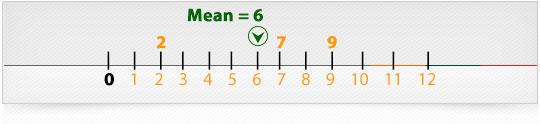
Example: what is the mean of 2, 7, and 9?
Add the numbers: 2 + 7 + 9 = 18
Divide by how many numbers (i.e., we added 3 numbers): 18 ÷ 3 = 6
So the Mean is 6

SAMPLE VARIANCE:

• Determine the mean

• Then for each number: subtract the Mean and square the result

• Then work out the mean of those squared differences.

To work out the mean, add up all the values then divide by the number of data points.

First add up all the values from the previous step.

But how do we say "add them all up" in mathematics? We use the Roman letter Sigma: Σ

The handy Sigma Notation says to sum up as many terms as we want.

• Next we need to divide by the number of data points, which is simply done by multiplying by "1/N":

Statistically it can be stated by the following:

• 

• This value is the variance

EXAMPLE:

The number of flowers on each bush is

9, 2, 5, 4, 12, 7, 8, 11, 9, 3, 7, 4, 12, 5, 4, 10, 9, 6, 9, 4

Work out the sample variance

Step 1. Work out the mean

In the formula above, μ (the Greek letter "mu") is the mean of all our values.

For this example, the data points are: 9, 2, 5, 4, 12, 7, 8, 11, 9, 3, 7, 4, 12, 5, 4, 10, 9, 6, 9, 4

The mean is:

(9+2+5+4+12+7+8+11+9+3+7+4+12+5+4+10+9+6+9+4) / 20 = 140/20 = 7

So:

μ = 7

Step 2. Then for each number: subtract the Mean and square the result

This is the part of the formula that says:

So what is xi? They are the individual x values 9, 2, 5, 4, 12, 7, etc...

In other words x1 = 9, x2 = 2, x3 = 5, etc.

So it says "for each value, subtract the mean and square the result", like this

Example (continued):

(9 - 7)2 = (2)2 = 4

(2 - 7)2 = (-5)2 = 25

(5 - 7)2 = (-2)2 = 4

(4 - 7)2 = (-3)2 = 9

(12 - 7)2 = (5)2 = 25

(7 - 7)2 = (0)2 = 0

(8 - 7)2 = (1)2 = 1

We need to do this for all the numbers

Step 3. Then work out the mean of those squared differences.

To work out the mean, add up all the values then divide by how many.

First add up all the values from the previous step.

= 4+25+4+9+25+0+1+16+4+16+0+9+25+4+9+9+4+1+4+9 = 178

But that isn't the mean yet, we need to divide by how many, which is simply done by multiplying by "1/N":

Mean of squared differences = (1/20) × 178 = 8.9

This value is called the variance.

STANDARD DEVIAITON:

DEFINITION:

This descriptor shows how much variation or dispersion from the average exists.

The symbol for Standard Deviation is σ (the Greek letter sigma).

It is calculated using:

In case of a sample the ‘N’ in this formula is replaced by n-1.

WHAT IT IS USED FOR:

It is used to determine the expected value. A low standard deviation indicates that the data points tend to be very close to the mean (also called expected value); a high standard deviation indicates that the data points are spread out over a large range of values.

HOW TO CALCULATE IT:

To determine the standard deviation, you need to take the square root of the variance.

EXAMPLE PROBLEM:

Let’s look at the previous problem and compute the standard deviation. The standard deviation as mentioned earlier is nothing more than the measure of dispersion (spread). It can be calculated by taking the square root of the variance. In case of the previous problem where the variance was 8.9, its corresponding standard deviation would be the square root of 8.9 which is 2.983

HYPOTHESES TESTING:

DEFINITION:

Hypothesis testing is a topic at the heart of statistics. This technique belongs to a realm known as inferential statistics. Researchers from all sorts of different areas, such as psychology, marketing, and medicine, formulate hypotheses or claims about a population being studied.

WHAT IT IS USED FOR:

Hypothesis testing is used to determine the validity of these claims. Carefully designed statistical experiments obtain sample data from the population. The data is in turn used to test the accuracy of a hypothesis concerning a population. Hypothesis tests are based upon the field of mathematics known as probability. Probability gives us a way to quantify how likely it is for an event to occur. The underlying assumption for all inferential statistics deals with rare events, which is why probability is used so extensively. The rare event rule states that if an assumption is made and the probability of a certain observed event is very small, then the assumption is most likely incorrect.

The basic idea here is that we test a claim by distinguishing between two different things:

1. An event that easily occurs by chance

2. An event that is highly unlikely to occur by chance.

If a highly unlikely event occurs, then we explain this by stating that a rare event really did take place, or that the assumption we started with was not true.

HOW TO USE THE TEST FOR DECISION MAKING PURPOSES:

1. Formulate the null hypothesis (commonly, that the observations are the result of pure chance) and the alternative hypothesis (commonly, that the observations show a real effect combined with a component of chance variation).

2. Identify a test statistic that can be used to assess the truth of the null hypothesis.

3. Compute the P-value, which is the probability that a test statistic at least as significant as the one observed would be obtained assuming that the null hypothesis were true. The smaller the -value, the stronger the evidence against the null hypothesis.

4. Compare the -value to an acceptable significance value (sometimes called an alpha value). If , that the observed effect is statistically significant, the null hypothesis is ruled out, and the alternative hypothesis is valid.

EXAMPLE OF HYPOTHESIS TESTING (TWO-TAIL TEST)

If you are told that the mean weight of 3rd graders is 85 pounds with a standard deviation of 20 pounds, and you find that the mean weight of a group of 22 students is 95 pounds, do you question that that group of students is a group of third graders?

• The z-score is ((x-bar) - µ)/(*sigma*/(n^.5)); the numerator is the difference between the observed and hypothesized mean, the denominator rescales the unit of measurement to standard deviation units. (95-85)/(20/(22^.5)) = 2.3452.

• The z-score 2.35 corresponds to the probability .9906, which leaves .0094 in the tail beyond. Since one could have been as far below 85, the probability of such a large or larger z-score is .0188. This is the p-value. Note that for these two tailed tests we are using the absolute value of the z-score.

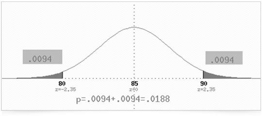
• Because .0188 < .05, we reject the hypothesis (which we shall call the null hypothesis) at the 5% significance level; if the null hypothesis were true, we would get such a large z-score less than 5% of the time. Because .0188 > .01, we fail to reject the null hypothesis at the 1% level; if the null hypothesis were true, we would get such a large z-score more than 1% of the time.

DECISION TREE:

DEFINITION:

A schematic tree-shaped diagram used to determine a course of action or show a statistical probability. Each branch of the decision tree represents a possible decision or occurrence. The tree structure shows how one choice leads to the next, and the use of branches indicates that each option is mutually exclusive.

WHAT IT IS USED FOR:

A decision tree can be used to clarify and find an answer to a complex problem. The structure allows users to take a problem with multiple possible solutions and display it in a simple, easy-to-understand format that shows the relationship between different events or decisions. The furthest branches on the tree represent possible end results.

HOW TO APPLY IT:

1. As a starting point for the decision tree, draw a small square around the center of the left side of the paper. If the description is too large to fit the square, use legends by including a number in the tree and referencing the number to the description either at the bottom of the page or in another page.

2. Draw out lines (forks) to the right of the square box. Draw one line each for each possible solution to the issue, and describe the solution along the line. Keep the lines as far apart as possible to expand the tree later.

3. Illustrate the results or the outcomes of the solution at the end of each line. If the outcome is uncertain, draw a circle (chance node). If the outcome leads to another issue, draw a square (decision node). If the issue is resolved with the solution, draw a triangle (end node). Describe the outcome above the square or circle, or use legends, as appropriate.

4. Repeat steps 2 through 4 for each new square at the end of the solution lines, and so on until there are no more squares, and all lines have either a circle or blank ending.

5. The circles that represent uncertainty remain as they are. A good practice is to assign a probability value, or the chance of such an outcome happening.

Since it is difficult to predict at onset the number of lines and sub-lines each solution generates, the decision tree might require one or more redraws, owing to paucity of space to illustrate or represent options and/or sub-options at certain spaces.

It is a good idea to challenge and review all squares and circles for possible overlooked solutions before finalizing the draft.

EXAMPLE:

Your company is considering whether it should tender for two contracts (MS1 and MS2) on offer from a government department for the supply of certain components. The company has three options:

• tender for MS1 only; or

• tender for MS2 only; or

• tender for both MS1 and MS2.

If tenders are to be submitted, the company will incur additional costs. These costs will have to be entirely recouped from the contract price. The risk, of course, is that if a tender is unsuccessful, the company will have made a loss.

The cost of tendering for contract MS1 only is $50,000. The component supply cost if the tender is successful would be $18,000.

The cost of tendering for contract MS2 only is $14,000. The component supply cost if the tender is successful would be $12,000.

The cost of tendering for both contracts MS1 and MS2 is $55,000. The component supply cost if the tender is successful would be $24,000.

For each contract, possible tender prices have been determined. In addition, subjective assessments have been made of the probability of getting the contract with a particular tender price as shown below. Note here that the company can only submit one tender and cannot, for example, submit two tenders (at different prices) for the same contract.

Option Possible Probability

tender of getting

prices ($) contract

MS1 only 130,000 0.20

115,000 0.85

MS2 only 70,000 0.15

65,000 0.80

60,000 0.95

MS1 and MS2 190,000 0.05

140,000 0.65

In the event that the company tenders for both MS1 and MS2 it will either win both contracts (at the price shown above) or no contract at all.

• What do you suggest the company should do and why?

• What are the downside and the upside of your suggested course of action?

• A consultant has approached your company with an offer that in return for $20,000 in cash, she will ensure that if you tender $60,000 for contract MS2, only your tender is guaranteed to be successful. Should you accept her offer or not and why?

Solution

The decision tree for the problem is shown below.

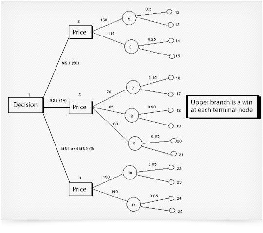
Below we carry out step 1 of the decision tree solution procedure which (for this example) involves working out the total profit for each of the paths from the initial node to the terminal node (all figures in $'000).

Step 1

• path to terminal node 12, we tender for MS1 only (cost 50), at a price of 130, and win the contract, so incurring component supply costs of 18, total profit 130-50-18 = 62

• path to terminal node 13, we tender for MS1 only (cost 50), at a price of 130, and lose the contract, total profit -50

• path to terminal node 14, we tender for MS1 only (cost 50), at a price of 115, and win the contract, so incurring component supply costs of 18, total profit 115-50-18 = 47

• path to terminal node 15, we tender for MS1 only (cost 50), at a price of 115, and lose the contract, total profit -50

• path to terminal node 16, we tender for MS2 only (cost 14), at a price of 70, and win the contract, so incurring component supply costs of 12, total profit 70-14-12 = 44

• path to terminal node 17, we tender for MS2 only (cost 14), at a price of 70, and lose the contract, total profit -14

• path to terminal node 18, we tender for MS2 only (cost 14), at a price of 65, and win the contract, so incurring component supply costs of 12, total profit 65-14-12 = 39

• path to terminal node 19, we tender for MS2 only (cost 14), at a price of 65, and lose the contract, total profit -14

• path to terminal node 20, we tender for MS2 only (cost 14), at a price of 60, and win the contract, so incurring component supply costs of 12, total profit 60-14-12 = 34

• path to terminal node 21, we tender for MS2 only (cost 14), at a price of 60, and lose the contract, total profit -14

• path to terminal node 22, we tender for MS1 and MS2 (cost 55), at a price of 190, and win the contract, so incurring component supply costs of 24, total profit 190-55- 24=111

• path to terminal node 23, we tender for MS1 and MS2 (cost 55), at a price of 190, and lose the contract, total profit -55

• path to terminal node 24, we tender for MS1 and MS2 (cost 55), at a price of 140, and win the contract, so incurring component supply costs of 24, total profit 140-55- 24=61

• path to terminal node 25, we tender for MS1 and MS2 (cost 55), at a price of 140, and lose the contract, total profit -55

Hence we can arrive at the table below indicating for each branch the total profit involved in that branch from the initial node to the terminal node.

Terminal node Total profit $'000

12 62

13 -50

14 47

15 -50

16 44

17 -14

18 39

19 -14

20 34

21 -14

22 111

23 -55

24 61

25 -55

We can now carry out the second step of the decision tree solution procedure where we work from the right-hand side of the diagram back to the left-hand side.

Step 2

• For chance node 5 the EMV is 0.2(62) + 0.8(-50) = -27.6

• For chance node 6 the EMV is 0.85(47) + 0.15(-50) = 32.45

Hence the best decision at decision node 2 is to tender at a price of 115 (EMV=32.45).

• For chance node 7 the EMV is 0.15(44) + 0.85(-14) = -5.3

• For chance node 8 the EMV is 0.80(39) + 0.20(-14) = 28.4

• For chance node 9 the EMV is 0.95(34) + 0.05(-14) = 31.6

Hence the best decision at decision node 3 is to tender at a price of 60 (EMV=31.6).

• For chance node 10 the EMV is 0.05(111) + 0.95(-55) = -46.7

• For chance node 11 the EMV is 0.65(61) + 0.35(-55) = 20.4

Hence the best decision at decision node 4 is to tender at a price of 140 (EMV=20.4).

Hence at decision node 1 we have three alternatives:

• tender for MS1 only EMV=32.45

• tender for MS2 only EMV=31.6

• tender for both MS1 and MS2 EMV = 20.4

Hence the best decision is to tender for MS1 only (at a price of 115) as it has the highest expected monetary value of 32.45 ($'000).

INFLUENCE OF SAMPLE SIZE:

DEFINITION:

Sample size is one of the four interrelated features of a study design that can influence the detection of significant differences, relationships, or interactions. Generally, these survey designs try to minimize both alpha error (finding a difference that does not actually exist in the population) and beta error (failing to find a difference that actually exists in the population).

WHAT IT IS USED FOR:

The sample size used in a study is determined based on the expense of data collection and the need to have sufficient statistical power.

HOW TO USE IT:

We already know that the margin of error is 1.96 times the standard error and that the standard error is sq.rt ^p(1