BUS 308 Discussion Questions 1 & 2
Week 5 Lecture 14
The Chi Square Test
Quite often, patterns of responses or measures give us a lot of information. Patterns are generally the result of counting how many things fit into a particular category. Whenever we make a histogram, bar, or pie chart we are looking at the pattern of the data. Frequently, changes in these visual patterns will be our first clues that things have changed, and the first clue that we need to initiate a research study (Lind, Marchel, & Wathen, 2008).
One of the most useful test in examining patterns and relationships in data involving counts (how many fit into this category, how many into that, etc.) is the chi-square. It is extremely easy to calculate and has many more uses than we will cover. Examining patterns involves two uses of the Chi-square - the goodness of fit and the contingency table. Both of these uses have a common trait: they involve counts per group. In fact, the chi-square is the only statistic we will look at that we use when we have counts per multiple groups (Tanner & Youssef-Morgan, 2013).
Chi Square Goodness of Fit TestThe goodness of fit test checks to see if the data distribution (counts per group) matches some pattern we are interested in. Example: Are the employees in our example company distributed equal across the grades? Or, a more reasonable expectation for a company might be are the employees distributed in a pyramid fashion – most on the bottom and few at the top?
The Chi Square test compares the actual versus a proposed distribution of counts by generating a measure for each cell or count: (actual – expected)2/actual. Summing these for all of the cells or groups provides us with the Chi Square Statistic. As with our other tests, we determine the p-value of getting a result as large or larger to determine if we reject or not reject our null hypothesis. An example will show the approach using Excel.
Regardless of the Chi Square test, the chi square related functions are found in the fx Statistics window rather than the Data Analysis where we found the t and ANOVA test functions. The most important for us are:
CHISQ.TEST (actual range, expected range) – returns the p-value for the test
CHISQ.INV.RT(p-value, df) – returns the actual Chi Square value for the p-value or probability value used.
CHISQ.DIST.RT(X, df) – returns the p-value for a given value.
When we have a table of actual and expected results, using the =CHISQ.TEST(actual range, expected range) will provide us with the p-value of the calculated chi square value (but does not give us the actual calculated chi square value for the test). We can compare this value against our alpha criteria (generally 0.05) to make our decision about rejecting or not rejecting the null hypothesis.
If, after finding the p-value for our chi square test, we want to determine the calculated value of the chi square statistic, we can use the =CHISQ.INV.RT(probability, df) function, the value for probability is our chi square test outcome, and the degrees of freedom (df) equals the number of cells in our actual table minus 1 (6 – 1 =5 for an problem working with our 6 grade levels). Finally, if we are interested in the probability of exceeding a particular chi square value, we can use the CHIDIST or CHISQ.DIST.RT function.
Excel Example. To see if our employees are distributed in a traditional pyramid shape, we would use the Chi Square Goodness of Fit test as we are dealing both with count data and with a proposed distribution pattern. For this test, let us assume the following table shows the expected distribution of our 50 employees in a pyramid organizational structure.
| A | B | C | D | E | F |
| 15 | 12 | 10 | 6 | 4 | 3 |
Grade: Total
Count: 50
The actual or observed distribution within our sample is shown below.
| A | B | C | D | E | F |
| 15 | 7 | 5 | 5 | 12 | 6 |
Grade: Total
Count: 50
The research question: Are employees distributed in a pyramidal fashion?
Step 1: Ho: No difference exists between observed and expected frequency counts Ha: Observed and Expected frequencies differ.
Step 2: Reject the null hypothesis if the p-value < alpha = .05.
Step 3: Chi Square Goodness of Fit test.
Step 4: Conduct the test. Below is a screen short of an Excel solution.
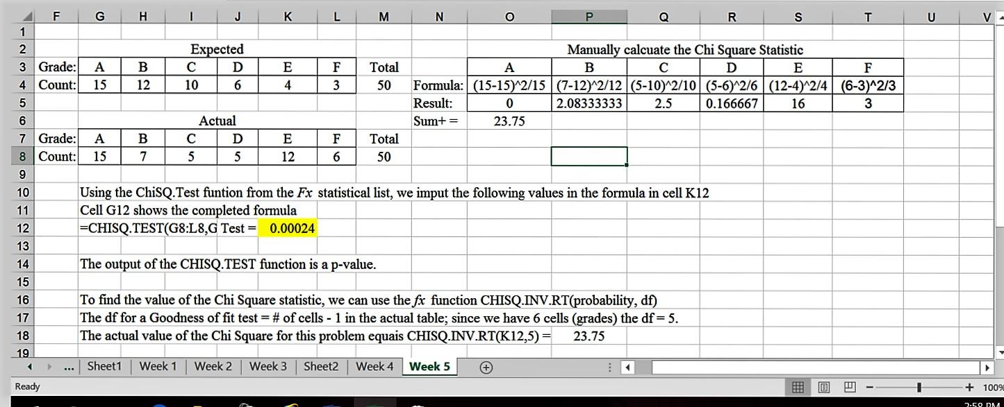
Step 5: Conclusions and Interpretation. Since our p-value of 0.00024 is < our alpha of 0.05, we reject the null hypothesis. The employees are not distributed in a pyramid pattern.
Side Note: We might think that if our sample had an equal number of employees per grade we would have a better chance of grade based differences averaging out. Doing this same test and assuming an equal distribution across grades produces a p-value of 0.063 causing us to fail to reject the null hypothesis. The student is encouraged to try this, the equal value for each grade would be 50/6.
Effect size. For a single row, goodness-of-fit test, the associated effect size measure is called effect size r, and equals the square root of: the chi square value/(N*df), where df = the number of cells – 1. A value less than .30 is considered small, between .30 and .50 is considered moderate, and more than .50 is considered large (Steinberg, 2008). Since we rejected the null in the example above, the effect size would be: r= square root (23.75/50*5) = sgrt(0.095) =0.31. This is a moderate impact, suggesting that both sample size and variable interaction had some impact. With moderate results, we generally would want to get a larger sample and repeat the test (Tanner & Youssef-Morgan, 2013).
Chi Square Contingency Table testContingency table tests, also known as tests of independence, are slightly more complex than goodness of fit tables. They classify the data by two or more variable labels (we will limit our discussions to two variable tables). Looking a lot like the input table for the ANOVA 2factor without replication we looked at last week. Both variables involve the counts per category (nominal, ordinal, or interval/ratio data in ranges) of items that meet our research interest (Lind, Marchel, & Wathen, 2008).
With most contingency tables, we do not have a given expected frequency as we had with the goodness of fit situation. To find the expected value for each cell for a multiple row/column table, we use the formula: row total * column total/grand total (which suggests the expected frequency is the average of the observed frequencies per cell, not an unreasonable expectation). Once we have generated the values for the expected table, we use the same formula to perform the Chi Square test. Manually, this is the sum of ((actual – expected)2/expected) for all of the cells. The same fx Chi Square functions used for the Goodness of Fit test are used for the Contingency Table analysis.
The null hypothesis for a contingency table test is “no relationship exists between the variables.” The alternate hypothesis would be: “a relationship exists.” In general, you are testing either for similar distributions between the groups of interest or to see if a relationship ("correlation") exists (even if the data is nominal level). The df for a contingency table is (number of rows-1)*(number of columns – 1).
Excel Example. The data entry for this test is the same as with our earlier test, and the functions are found in the fx statistical list. One possible explanation for different salaries is the performance on the job, reflected in the performance rating. We might wonder if males and females are evaluated differently (either due to actual performance or to bias; if so, we have another issue to examine). So, our research question for this issue becomes, are males and females rated the same?
Step 1: Ho: Male and Female ratings are similar (no difference in distributions)
Ha: Males and Females rating distributions differ Step 2: Reject Ho if p-value is < alpha = 0.05. Step 3: Chi Square Contingency Table Analysis Step 4: Perform Test.
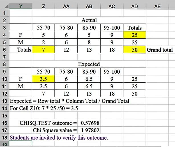
Step 5: Conclusions and Interpretation. Since the p-value (CHISQ.TEST result) is greater than
(>) alpha = .05, we fail to reject the null hypothesis and conclude that males and females are evaluated in a similar pattern. It does not appear that performance rating impact average salary differences.
Effect size. Now, as with the t-test and ANOVA, had we rejected the null hypothesis, we would have wanted to examine the practical impact of the outcome using an effect size measure. The effect size measure for the Chi Square is a correlation measure. Two measures are generally used with the contingency table outcomes – the Phi coefficient and Cramer’s V (Tanner & Youssef-Morgan, 2013).
The Phi coefficient (=square root of (chi square/sample size)) provides a rough estimate of the correlation between the two variables. Phi is primarily used with small tables (2x2, 2x3, or 3x2). Values below .30 are weak, .30 to about .50 are moderate, and above .50 (to 1) are strong relationships (Tanner & Youssef-Morgan, 2013).
Cramer’s V can be considered as a percent of the shared variation – or common variation between the variables. It equals the square root of (phi squared/(smaller number of rows or columns -1). It ranges from 0 (no relationship or variation in common) to 1.0 (strong relationship, all variation in common) (Tanner & Youssef-Morgan, 2013).
For our example above, it would not make sense to calculate either value since we did not reject the null; but for illustrative purposes we will.
Phi = square root of (1.978/50) = square root of (0.03956) = 0.199 –small, no relationship
V = square root of (0.1.99^2/(2-1)) = 0.19. Note, when the smaller of the number of rows and columns equals 1, V will equal Phi (Tanner & Youssef-Morgan, 2013).
Due to the division involved in calculating the Chi Square value, it is extremely influenced with cells that have small expected values. Most texts say simply that if the expected frequency in one or more cells is less than (<) 5 to not use the Chi Square distribution in a hypothesis test. There are some different opinions about this issue. Different texts issue different rules on what to do if we have expected frequencies of 5 or less in cells.
As a compromise, let’s use the standard that no more than 20% of the cells should have an expected value of less than 5. If they do, we need to combine rows or columns to reduce this percentage interest (Lind, Marchel, & Wathen, 2008).
References
Lind, D. A., Marchel, W. G., & Wathen, S. A. (2008). Statistical Techniques in Business & Finance. (13th Ed.) Boston: McGraw-Hill Irwin.
Steinberg, W.J. (2008). Statistics Alive! Thousand Oaks, CA: Sage Publications, Inc.
Tanner, D. E. & Youssef-Morgan, C. M. (2013). Statistics for Managers. San Diageo, CA: Bridgeport Education.


