Discussion/ Chapter Summary Chapters 10,11 and 20

Chapter 11- Cash Flow Estimation and Risk Analysis

Chapter Introduction

Procter & Gamble, Unilever, and the Thales Group are among the many companies that understand the importance of cash flow estimation and risk analysis. For example, P&G conducts risk analysis on a wide variety of capital budgeting projects, from routine cost savings proposals at domestic facilities to cross-border facility location choices. P&G’s Associate Director for Investment Analysis, Bob Hunt, says that risk analysis, especially the use of decision trees, “has been very useful in helping us break complex projects down into individual decision options, helping us understand the uncertainties, and ultimately helping us make superior decisions.”

Unilever created its Decision Making Under Uncertainty () approach to avoid overlooking risk during its project selection process. Unilever applies DMUU to conduct risk analysis for many types of projects, but especially when it must choose among multiple proposals.

Project evaluation is always difficult, but it is even more so when rapidly evolving technology is involved. For firms bidding for government and business contracts, the bidding process itself ramps up the already difficult task of project evaluation. The Thales Group competes in this market by providing communication systems for the defense and aerospace industries. Not only does Thales use risk analysis to better identify the expected levels and risks of project cash flows, but it also uses risk analysis to better understand and manage the risks associated with submitting bids for projects.

Keep these companies in mind as you read the chapter.

Source: Palisade Corporation is a leading developer of software for risk evaluation and decision analysis. For examples of companies using risk analysis, see the case analyses at www.palisade.com/cases.

Project Valuation, Cash Flows, and Risk Analysis

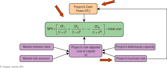
When we estimate a project’s cash flows () and then discount them at the project’s risk-adjusted cost of capital, r, the result is the project’s NPV, which tells us how much the project increases the firm’s value. This chapter focuses on how to estimate the size and risk of a project’s cash flows.

Note too that project cash flows, once a project has been accepted and placed in operation, are added to the firm’s free cash flows from other sources. Therefore, projects’ cash flows essentially determine the firm’s free cash flows as discussed in Chapter 2 and thus form the basis for the firm’s market value and stock price.

© Cengage Learning 2014

Resource

The textbook’s Web site contains an Excel file that will guide you through the chapter’s calculations. The file for this chapter is ch11 Tool Kit.xls, and we encourage you to open the file and follow along as you read the chapter.

Chapter 10 assumed that a project’s cash flows had already been estimated. Now we cover cash flow estimation and identify the issues a manager faces in producing relevant and realistic cash flow estimates. In addition, cash flow estimates are just that: estimates! It is crucial for a manager to incorporate uncertainty into project analysis if a company is to make informed decisions regarding project selection. We begin with a discussion of procedures for estimating relevant and realistic cash flows.

11-1

Identifying Relevant Cash Flows

The most important—and difficult—step in capital budgeting is estimating a proposal’s relevant project cash flows, which are the differences between the cash flows the firm will have if it implements the project versus the cash flows it will have if it rejects the project. These are called incremental cash flows:

Estimating incremental cash flows might sound easy, but there are many potential pitfalls. In this section, we identify the key concepts that will help you avoid these pitfalls and then apply the concepts to an actual project to illustrate their application to cash flow estimation.

11-1a

Cash Flow versus Accounting Income

We saw in Chapter 2 that free cash flow differs from accounting income: Free cash flow is cash flow that is available for distribution to investors, making free cash flow the basis of a firm’s value. It is common in the practice of finance to speak of a firm’s free cash flow and a project’s cash flow (or net cash flow), but these are based on the same concepts. In fact, a project’s cash flow is identical to the project’s free cash flow, and a firm’s total net cash flow from all projects is equal to the firm’s free cash flow. We will follow the typical convention and refer to a project’s free cash flow simply as project cash flow, but keep in mind that the two concepts are identical.

Because net income is not equal to the cash flow available for distribution to investors, in the last chapter we discounted net cash flows, not accounting income, to find projects’ . For capital budgeting purposes it is the project’s net cash flow, not its accounting income, which is relevant. Therefore, when analyzing a proposed capital budgeting project, disregard the project’s net income and focus exclusively on its net cash flow. Be especially alert to the following differences between cash flow and accounting income.

The Cash Flow Effect of Asset Purchases and Depreciation

Most projects require assets, and asset purchases represent negative cash flows. Even though the acquisition of assets results in a cash outflow, accountants do not show the purchase of fixed assets as a deduction from accounting income. Instead, they deduct a depreciation expense each year throughout the life of the asset. Depreciation shelters income from taxation, and this has an impact on cash flow, but depreciation itself is not a cash flow. Therefore, depreciation must be added back when estimating a project’s operating cash flow.

Depreciation is the most common noncash charge, but there are many other noncash charges that might appear on a company’s financial statements. Just as with depreciation, all other noncash charges should be added back when calculating a project’s net cash flow.

Changes in Net Operating Working Capital

Normally, additional inventories are required to support a new operation, and expanded sales tie up additional funds in accounts receivable. However, payables and accruals increase as a result of the expansion, and this reduces the cash needed to finance inventories and receivables. The difference between the required increase in operating current assets and the increase in operating current liabilities is the change in net operating working capital. If this change is positive, as it generally is for expansion projects, then additional financing—beyond the cost of the fixed assets— will be needed.

Toward the end of a project’s life, inventories will be used but not replaced, and receivables will be collected without corresponding replacements. As these changes occur the firm will receive cash inflows; as a result, the investment in net operating working capital will be returned by the end of the project’s life.

Interest Charges are Not Included in Project Cash Flows

Interest is a cash expense, so at first blush it would seem that interest on any debt used to finance a project should be deducted when we estimate the project’s net cash flows. However, this is not correct. Recall from Chapter 10 that we discount a project’s cash flows by its risk-adjusted cost of capital, which is a weighted average () of the costs of debt, preferred stock, and common equity, adjusted for the project’s risk and debt capacity. This project cost of capital is the rate of return necessary to satisfy all of the firm’s investors, including stockholders and debtholders. A common mistake made by many students and financial managers is to subtract interest payments when estimating a project’s cash flows. This is a mistake because the cost of debt is already embedded in the cost of capital, so subtracting interest payments from the project’s cash flows would amount to double-counting interest costs. Therefore, you should not subtract interest expenses when finding a project’s cash flows.

11-1bTiming of Cash Flows: Yearly versus Other Periods

In theory, in capital budgeting analyses we should discount cash flows based on the exact moment when they occur. Therefore, one could argue that daily cash flows would be better than annual flows. However, it would be costly to estimate daily cash flows and laborious to analyze them. In general the analysis would be no better than one using annual flows because we simply can’t make accurate forecasts of daily cash flows more than a couple of months into the future. Therefore, it is generally appropriate to assume that all cash flows occur at the end of the various years. For projects with highly predictable cash flows, such as constructing a building and then leasing it on a long-term basis (with monthly payments) to a financially sound tenant, we would analyze the project using monthly periods.

11-1cExpansion Projects and Replacement Projects

Two types of projects can be distinguished: 

• (1)

expansion projects, in which the firm makes an investment in, for example, a new Home Depot store in Seattle; and

• (2)

replacement projects, in which the firm replaces existing assets, generally to reduce costs.

In expansion projects, the cash expenditures on buildings, equipment, and required working capital are obviously incremental, as are the sales revenues and operating costs associated with the project. The incremental costs associated with replacement projects are not so obvious. For example, Home Depot might replace some of its delivery trucks to reduce fuel and maintenance expenses. Replacement analysis is complicated by the fact that most of the relevant cash flows are the cash flow differences between the existing project and the replacement project. For example, the fuel bill for a more efficient new truck might be  versus  for the old truck, and the  fuel savings would be an incremental cash flow associated with the replacement decision. We analyze an expansion and replacement decision later in the chapter.

A sunk cost is an outlay related to the project that was incurred in the past and that cannot be recovered in the future regardless of whether or not the project is accepted. Therefore, sunk costs are not incremental costs and thus are not relevant in a capital budgeting analysis.

To illustrate, suppose Home Depot spent  to investigate sites for a potential new store in a given area. That  is a sunk cost—the money is gone, and it won’t come back regardless of whether or not a new store is built. Therefore, the should not be included in a capital budgeting decision. Improper treatment of sunk costs can lead to bad decisions. For example, suppose Home Depot completed the analysis for a new store and found that it must spend an additional (or incremental)  to build and supply the store, on top of the  already spent on the site study. Suppose the present value of future cash flows is  . Should the project be accepted? If the sunk costs are mistakenly included, the  is  and the project would be rejected. However, that would be a bad decision. The real issue is whether the incremental would result in enough incremental cash flow to produce a positive NPV. If the  sunk cost were disregarded, as it should be, then the  on an incremental basis would be a positive  .

Another conceptual issue relates to opportunity costs related to assets the firm already owns. Continuing our example, suppose Home Depot () owns land with a current market value of  that can be used for the new store if it decides to build the store. If HD goes forward with the project, only another  will be required, not the full  , because it will not need to buy the required land. Does this mean that HD should use the  incremental cost as the cost of the new store? The answer is definitely “no.” If the new store is not built, then HD could sell the land and receive a cash flow of  . This  is an opportunity cost—it is cash that HD would not receive if the land is used for the new store. Therefore, the  must be charged to the new project, and failing to do so would cause the new project’s calculated  to be too high.

Another conceptual issue relates to externalities, which are the effects of a project on other parts of the firm or on the environment. As explained in what follows, there are three types of externalities: negative within-firm externalities, positive within-firm externalities, and environmental externalities.

If a retailer like Home Depot opens a new store that is close to its existing stores, then the new store might attract customers who would otherwise buy from the existing stores, reducing the old stores’ cash flows. Therefore, the new store’s incremental cash flow must be reduced by the amount of the cash flow lost by its other units. This type of externality is called cannibalization, because the new business eats into the company’s existing business. Many businesses are subject to cannibalization. For example, each new iPod model cannibalizes existing models. Those lost cash flows should be considered, and that means charging them as a cost when analyzing new products.

Dealing properly with negative externalities requires careful thinking. If Apple decided not to come out with a new model of iPod because of cannibalization, another company might come out with a similar new model, causing Apple to lose sales on existing models.

Apple must examine the total situation, and this is definitely more than a simple, mechanical analysis. Experience and knowledge of the industry is required to make good decisions in most cases.

One of the best examples of a company getting into trouble as a result of not dealing correctly with cannibalization was IBM’s response to the development of the first personal computers in the 1970s. IBM’s mainframes dominated the computer industry, and they generated huge profits. IBM used its technology to enter the PC market, and initially it was the leading PC company. However, its top managers decided to deemphasize the PC division because they were afraid it would hurt the more profitable mainframe business. That decision opened the door for Apple, Dell, Hewlett Packard, Sony, and Chinese competitors to take PC business away from IBM. As a result, IBM went from being the most profitable firm in the world to one whose very survival was threatened. IBM’s experience highlights that it is just as important to understand the industry and the long-run consequences of a given decision as it is to understand the theory of finance. Good judgment is an essential element for good financial decisions.

As we noted earlier, cannibalization occurs when a new product competes with an old one. However, a new project can also be complementary to an old one, in which case cash flows in the old operation will be increased when the new one is introduced. For example, Apple’s iPod was a profitable product, but when Apple considered an investment in its music store it realized that the store would boost sales of iPods. So, even if an analysis of the proposed music store indicated a negative NPV, the analysis would not be complete unless the incremental cash flows that would occur in the iPod division were credited to the music store. Consideration of positive externalities often changes a project’s  from negative to positive.

The most common type of negative externality is a project’s impact on the environment. Government rules and regulations constrain what companies can do, but firms have some flexibility in dealing with environmental issues. For example, suppose a manufacturer is studying a proposed new plant. The company could meet current environmental regulations at a cost of  , but the plant would still emit fumes that would cause some bad will in its neighborhood. Those ill feelings would not show up in the cash flow analysis, but they should be considered. Perhaps a relatively small additional expenditure would reduce the emissions substantially, make the plant look good relative to other plants in the area, and provide goodwill that in the future would help the firm’s sales and its negotiations with governmental agencies.

Of course, all firms’ profits ultimately depend on the Earth remaining healthy, so companies have some incentive to do things that protect the environment even though those actions are not currently required. However, if one firm decides to take actions that are good for the environment but quite costly, then it must either raise its prices or suffer a decline in earnings. If its competitors decide to get by with less costly but environmentally unfriendly processes, they can price their products lower and make more money. Of course, the more environmentally friendly companies can advertise their environmental efforts, and this might—or might not—offset their higher costs. All this illustrates why government regulations are often necessary. Finance, politics, and the environment are all interconnected.

In Chapter 10, we worked with the cash flows associated with one of Guyton Products Company’s expansion projects. Recall that Project L is the application of a radically new liquid nano-coating technology to a new type of solar water heater module, which will be manufactured under a  license from a university. In this section we show how these cash flows are estimated (we only show estimates for Project L in the chapter, but we also show estimates GPC’s other project from Chapter 10, Project S, in ch11 Tool Kit.xls). It’s not clear how well the water heater will work, how strong demand for it will be, how long it will be before the product becomes obsolete, or whether the license can be renewed after the initial  . Still, the water heater has the potential for being profitable, though it could also fail miserably. GPC is a relatively large company and this is one of many projects, so a failure would not bankrupt the firm but would hurt profits and the stock’s price.

11-2a

Base Case Inputs and Key Results

Resource

See ch11 Tool Kit.xls on the textbook’s Web site.

We used Excel to do the analysis. We could have used a calculator and paper, but Excel is much easier when dealing with capital budgeting problems. You don’t need to know Excel to understand our discussion, but if you plan to work in finance—or, really, in any business field—you must know how to use Excel, so we recommend that you open the Excel Tool Kit for this chapter and scroll through it as the textbook explains the analysis.

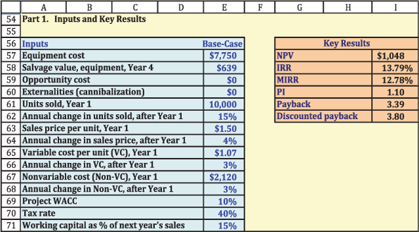
Figure 11-1 shows the Part 1 of the Excel model used in this analysis; see the first worksheet in ch11 Tool Kit.xls named 1-Base-Case . The base-case inputs are in the blue section. For example, the cost of required equipment to manufacture the water heaters is and is shown in the blue input section. (All dollar values in Figure 11-1 and in our discussion here are reported in thousands, so the equipment actually costs .) The actual number-crunching takes place in Part 2 of the model, shown in Figure 11-2. Part 2 takes the inputs from the blue section of Figure 11-1 and generates the project’s cash flows. Part 2 of the model also performs calculations of the project performance measures discussed in Chapter 10 and then reports those results in the orange section of Figure 11-1. This structure allows you (or your manager) to change and input and instantly see the impact on the reported performance measures.

Figure 11-1

Analysis of an Expansion Project: Inputs and Key Results (Thousands of Dollars)

Figure 11-2

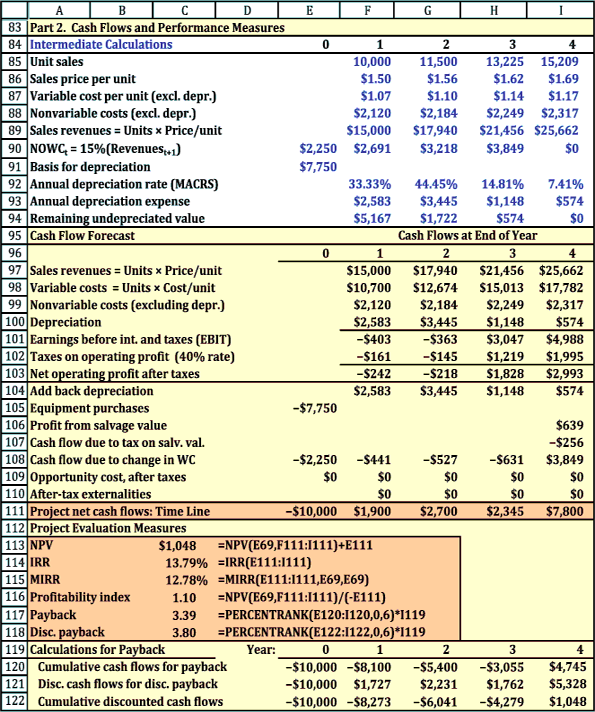
Analysis of an Expansion Project: Cash Flows and Performance Measures (Thousands of Dollars)

We have saved these base-case inputs in ch11 Tool Kit.xls with Excel’s Scenario Manager. If you change some inputs but want to return to the original base-case inputs, you can select Data, What-If Analysis, Scenario Manager, pick the scenario named “Base-Case for Project L,” and click Show. This will replace any changes with the original inputs. Scenario Manager is a very useful tool and we will have more to say about it later in this chapter.

11-2b

Cash Flow Projections: Intermediate Calculations

Resource

See ch11 Tool Kit.xls on the textbook’s Web site.

Figure 11-2 shows Part 2 of the model. When setting up Excel models, we prefer to have more rows but shorter formulas. So instead of having very complicated formulas in the section for cash flow forecasts, we put intermediate calculations in a separate section. The blue section of Figure 11-2 shows these intermediate calculations for the GPC project, as we explain in the following sections.

Annual Unit Sales, Unit Prices, Unit Costs, and Inflation

Rows 85–88 show annual unit sales, unit sale prices, unit variable costs, and nonvariable costs. These values are all projected to grow at the rates assumed in Part 1 of the model in Figure 11-1. If you ignore growth in prices and costs when estimating cash flows, you are likely to underestimate a project’s value because the project’s weighted average cost of capital () includes the impact of inflation. In other words, the estimated cash flows will be too low relative to the , so the estimated net present value () also will be too low relative to the true NPV. To see that the includes inflation, recall from Chapter 5 that the cost of debt includes an inflation premium. Also, the capital asset pricing model from Chapter 6 defines the cost of equity as the sum of the risk-free rate and a risk premium. Like the cost of debt, the risk-free rate also has an inflation premium. Therefore, if the includes the impact of inflation, the estimated cash flows must also include inflation. It is theoretically possible to ignore inflation when estimating the cash flows but adjust the so that it, too, doesn’t incorporate inflation, but we have never seen this accomplished correctly in practice. Therefore, you should always include growth rates in prices and costs when estimating cash flows.

Net Operating Working Capital ()

Virtually all projects require working capital, and this one is no exception. For example, raw materials must be purchased and replenished each year as they are used. In Part 1 (Figure 11-1) we assume that GPC must have an amount of net operating working capital on hand equal to of the upcoming year’s sales. For example, in Year 0, GPC must have in working capital on hand. As sales grow, so does the required working capital. Rows 89–90 show the annual sales revenues (the product of units sold and sales price) and the required working capital.

Depreciation Expense

Resource

See ch11 Tool Kit.xls on the textbook’s Web site.

Rows 91–94 report intermediate calculations related to depreciation, beginning with the depreciation basis, which is the cost of acquiring and installing a project. The basis for GPC’s project is . The depreciation expense for a year is the product of the basis and that year’s depreciation rate. Depreciation rates depend on the type of property and its useful life. Even though GPC’s project will operate for , it is classified as property for tax purposes. The depreciation rates in Row 92 are for property using the modified cost accelerated cost recovery system (); see Appendix 11-A and the chapter’s Tool Kit for more discussion of depreciation. The remaining undepreciated value is equal to the original basis less the accumulated depreciation; this is called the book value of the asset and is used later in the model when calculating the tax on the salvage value.

11-2c

Cash Flow Projections: Estimating Net Operating Profit after Taxes ()

The yellow section in the middle of Figure 11-2 shows the steps in calculating the project’s net operating profit after taxes (). Projected sales revenues are on Row 97. Annual variable unit costs are multiplied by the number of units sold to determine total variable costs, as shown on Row 98. Nonvariable costs are shown on Row 99, and depreciation expense is shown on Row 100. Subtracting variable costs, nonvariable costs, and depreciation from sales revenues results in operating profit, as shown on Row 101.

When discussing a company’s income statement, operating profit often is called earnings before interest and taxes (). Remember, though, that we do not subtract interest when estimating a project’s cash flows, because the project’s is the overall rate of return required by all the company’s investors and not just shareholders. Therefore, the cash flows must also be the cash flows available to all investors and not just shareholders, so we do not subtract interest expense. We calculate taxes in Row 102 and subtract them to get the project’s net operating profit after taxes () on Row 103. The project has negative earnings before interest and taxes in Years 1 and 2. When multiplied by the tax rate, Row 102 shows negative taxes for Years 1 and 2. This negative tax is subtracted from EBIT and actually makes the after-tax operating profit larger than the pre-tax profit! For example, the Year 1 pre-tax profit is and the reported tax is , leading to an after-tax profit of . In other words, it is as though the IRS is sending GPC a check for . How can this be correct?

Recall the basic concept underlying the relevant cash flows for project analysis—what are the company’s cash flows with the project versus the company’s cash flows without the project? Applying this concept, if GPC expects to have taxable income from other projects in excess of in Year 1, then the project will shelter that income from in taxes. Therefore, the project will generate in cash flow for GPC in Year 1 due to the tax savings.

11-2d

Cash Flow Projections: Adjustments to NOPAT

Row 103 reports the project’s NOPAT, but we must adjust NOPAT to determine the project’s actual cash flows. In particular, we must account for depreciation, asset purchases and dispositions, changes in working capital, opportunity costs, externalities, and sunk costs.

Adjustments to Determine Cash Flows: Depreciation

The first step is to add back depreciation, which is a noncash expense. You might be wondering why we subtract depreciation on Row 100 only to add it back on Row 104, and the answer is due to depreciation’s impact on taxes. If we had ignored the Year 1 depreciation of when calculating NOPAT, the pre-tax income () for Year 1 would have been instead of . Taxes would have been instead of . This is a difference of . Cash flows should reflect the actual taxes, but we must add back the noncash depreciation expense to reflect the actual cash flow.

Adjustments to Determine Cash Flows: Asset Purchases and Dispositions

GPC purchased the asset at the beginning of the project for , which is a negative cash flow shown on Row 105. Had GPC purchased additional assets in other years, we would report those purchases, too.

GPC expects to salvage the investment at Year 4 for . In our example, GPC’s project was fully depreciated by the end of the project, so the salvage value is a taxable profit. At a tax rate, GPC will owe in taxes, as shown on Row 107.

Suppose instead that GPC terminates operations before the equipment is fully depreciated. The after-tax salvage value depends on the price at which GPC can sell the equipment and on the book value of the equipment (i.e., the original basis less all previous depreciation charges). Suppose GPC terminates at Year 2, at which time the book value is , as shown on Row 94. We consider two cases, gains and losses. In the first case, the salvage value is and so there is a reported gain of . This gain is taxed as ordinary income, so the tax is . The after-tax cash flow is equal to the sales price less the tax: .

Now suppose the salvage value at Year 2 is only . In this case, there is a reported loss: . This is treated as an ordinary expense, so its tax is . This “negative” tax acts as a credit if GPC has other taxable income, so the net after-tax cash flow is .

Adjustments to Determine Cash Flows: Working Capital

Row 90 shows the total amount of net operating working capital needed each year. Row 108 shows the incremental investment in working capital required each year. For example, at the start of the project, Cell E108 shows a cash flow of will be needed at the beginning of the project to support Year 1 sales. Row 90 shows working capital must increase from to to support Year 2 sales. Thus, GPC must invest in working capital in Year 1, and this is shown as a negative number (because it is an investment) in Cell F108. Similar calculations are made for Years 2 and 3. At the end of Year 4, all of the investments in working capital will be recovered. Inventories will be sold and not replaced, and all receivables will be collected by the end of Year 4. Total net working capital recovered at is the sum of the initial investment at , , plus the additional investments during Years 1 through 3; the total is .

Adjustments to Determine Cash Flows: Sunk Costs, Opportunity Costs, and Externalities

GPC’s project doesn’t have any sunk costs, opportunity costs, or externalities, but the following sections show how we would adjust the cash flows if GPC did have some of these issues.

Sunk Costs. Suppose that last year GPC spent on a marketing and feasibility study for the project. Should be included in the project’s cost? The answer is no. That money already has been spent and accepting or rejecting the project will not change that fact.

Opportunity Costs. Now suppose the equipment cost was based on the assumption that the project would use space in a building that GPC now owns but that the space could be leased to another company for , after taxes, if the project is rejected. The would be an opportunity cost, and it should be reflected in the cash flow calculations.

Externalities. As noted earlier, the solar water heater project does not lead to any cannibalization effects. Suppose, however, that it would reduce the net after-tax cash flows of another GPC division by and that no other firm could take on this project if GPC turns it down. In this case, we would use the cannibalization line at Row 110, deducting each year. As a result, the project would have a lower NPV. On the other hand, if the project would cause additional inflows to some other GPC division because it was complementary to that other division’s products (i.e., if a positive externality exists), then those after-tax inflows should be attributed to the water heater project and thus shown as a positive inflow on Row 110.

11-2e

Evaluating Project Cash Flows

We sum Rows 103 to 110 to get the project’s annual net cash flows, set up as a time line on Row 111. These cash flows are then used to calculate , , , , payback, and discounted payback, performance measures that are shown in the orange portion at the bottom of Figure 11-2.

Preliminary Evaluation of the Base-Case Scenario

Based on this analysis, the preliminary evaluation indicates that the project is acceptable. The is , which is fairly large when compared to the initial investment of . Its and are both greater than the , and the is larger than . The payback and discounted payback are almost as long as the project’s life, which is somewhat concerning, and is something that needs to be explored by conducting a risk analysis of the project.

Scenario Manager

Excel’s Scenario Manager is a very powerful and useful tool. We illustrate its use here as we examine two topics, the impact of forgetting to include inflation and the impact of accelerated depreciation versus straight-line depreciation. To use Scenario Manager in the worksheet named 1-Base-Case in ch11 Tool Kit.xls, Select Data, What-If Analysis, and Scenario Manager. There are five scenarios:

• (1)
Base-Case for Project L but Forget Inflation,

• (2)
Base-Case for Project L,

• (3)
Project S,

• (4)
MACRS Depreciation, and

• (5)
Straight-Line Depreciation.

The first three scenarios change the inputs in Rows 56–71. The last two scenarios change the depreciation rates in Row 92. This structure allows you to choose a set of inputs and then choose a depreciation method. Sometimes we include all the changing cells in each scenario, and sometimes we separate the scenarios into different groups as we did in this example.

The advantage of having all changing cells in each scenario is that you only have to select a single scenario to show all the desired inputs in the model. The disadvantage is that each scenario can get complicated by having many changing cells.

The advantage of having groups of scenarios is that you can focus on particular aspects of the analysis, such as the choice of depreciation methods. The disadvantage is that you must know which other scenarios are active in order to properly interpret your results.

For some models it makes sense to have only one group of scenarios in which each scenario has the same changing cells; for other models it makes sense to have different groups of scenarios.

The Impact of Inflation. It is easy to overlook inflation, but it is important to include it. For example, had we forgotten to include inflation in the GPC example, the estimated would have dropped from to . You can see this by changing all the price and cost growth rates to zero and then looking at the NPV. An easy way to do this is with the Scenario Manager—just choose the scenario named “Base-Case for Project L but Forget Inflation.” Forgetting to include inflation in a capital budgeting analysis typically causes the estimated to be lower than the true NPV, which could cause a company to reject a project that it should have accepted. You can return to the original inputs by going back into Scenario Manager, selecting “Base-Case for Project L,” and clicking on “Show.”

Accelerated Depreciation versus Straight-Line Depreciation. Congress permits firms to depreciate assets using either the straight-line method or an accelerated method. The results we have discussed thus far were based on accelerated depreciation. To see the impact of using straight-line depreciation, go to the Scenario Manager and select “Straight-Line Depreciation.” Be sure that you have also selected “Base-Case for Project L.” After selecting and showing these two scenarios, you will have a set of inputs for the base-case and straight-line deprecation rates.

The results indicate that the project’s is when using straight-line depreciation, which is lower than the when using accelerated depreciation. In general, profitable firms are better off using accelerated depreciation because more depreciation is taken in the early years under the accelerated method, so taxes are lower in those years and higher in later years. Total depreciation, total cash flows, and total taxes are the same under both depreciation methods, but receiving the cash earlier under the accelerated method results in a higher , , and .

Suppose Congress wants to encourage companies to increase their capital expenditures and thereby boost economic growth and employment. What changes in depreciation regulations would have the desired effect? The answer is “Make accelerated depreciation even more accelerated.” For example, if GPC could write off equipment at rates of , , , and rather than , , , and , then its early tax payments would be even lower, early cash flows would be even higher, and the project’s would exceed the value shown in Figure 11-2.

Be sure to return the scenarios to “Base-Case for Project L” and “MACRS Depreciation.”

Project S. Recall from Chapter 10 that GPC was also considering Project S, which used solid coatings. You can use the Scenario Manager to show this project by selecting the scenario “Project S,” which will show the cash flows used in Chapter 10. Be sure to return the scenarios in the worksheet 1-Base-Case to “Base-Case for Project L” and “MACRS Depreciation.”

11-3

Risk Analysis in Capital Budgeting

Projects differ in risk, and risk should be reflected in capital budgeting decisions. There are three separate and distinct types of risk.

• Stand-alone risk is a project’s risk assuming

  1. (a)
that it is the firm’s only asset and

  2. (b)
that each of the firm’s stockholders holds only that one stock in his portfolio.

• Standalone risk is based on uncertainty about the project’s expected cash flows. It is important to remember that stand-alone risk ignores diversification by both the firm and its stockholders.

• Within-firm risk (also called corporate risk) is a project’s risk to the corporation itself. Within-firm risk recognizes that the project is only one asset in the firm’s portfolio of projects; hence some of its risk is eliminated by diversification within the firm. However, within-firm risk ignores diversification by the firm’s stockholders.Within-firm risk is measured by the project’s impact on uncertainty about the firm’s future total cash flows.

• Market risk (also called beta risk) is the risk of the project as seen by a well- diversified stockholder who recognizes that

  1. (a)
the project is only one of the firm’s projects and

  2. (b)
the firm’s stock is but one of her stocks.

• The project’s market risk is measured by its effect on the firm’s beta coefficient.

Taking on a project with a lot of stand-alone and/or corporate risk will not necessarily affect the firm’s beta. However, if the project has high stand-alone risk and if its cash flows are highly correlated with cash flows on the firm’s other assets and with cash flows of most other firms in the economy, then the project will have a high degree of all three types of risk. Market risk is, theoretically, the most relevant because it is the one that, according to the CAPM, is reflected in stock prices. Unfortunately, market risk is also the most difficult to measure, primarily because new projects don’t have “market prices” that can be related to stock market returns.

Resource

See Web Extension 11A on the textbook’s Web site for a more detailed discussion on alternative methods for incorporating project risk into the capital budgeting decision process.

Most decision makers conduct a quantitative analysis of stand-alone risk and then consider the other two types of risk in a qualitative manner. They classify projects into several categories; then, using the firm’s overall as a starting point, they assign a risk-adjusted cost of capital to each category. For example, a firm might establish three risk classes and then assign the corporate to average-risk projects, add a risk premium for higher-risk projects, and subtract for low-risk projects. Under this setup, if the company’s overall were , then would be used to evaluate average-risk projects, for high-risk projects, and for low-risk projects. Although this approach is probably better than not making any risk adjustments, these adjustments are highly subjective and difficult to justify. Unfortunately, there’s no perfect way to specify how high or low the risk adjustments should be.

A project’s stand-alone risk reflects uncertainty about its cash flows. The required dollars of investment, unit sales, sales prices, and operating costs as shown in Figure 11-1 for GPC’s project are all subject to uncertainty. First-year sales are projected at units to be sold at a price of  per unit (recall that all dollar values are reported in thousands). However, unit sales will almost certainly be somewhat higher or lower than  , and the price will probably turn out to be different from the projected  per unit. Similarly, the other variables would probably differ from their indicated values. Indeed, all the inputs are expected values, not known values, and actual values can and do vary from expected values. That’s what risk is all about!

Three techniques are used in practice to assess stand-alone risk: 

• (1)

sensitivity analysis,

• (2)

scenario analysis, and

• (3)

Monte Carlo simulation.

We discuss them in the sections that follow.

Intuitively, we know that a change in a key input variable such as units sold or the sales price will cause the  to change. Sensitivity analysis measures the percentage change in  that results from a given percentage change in an input variable when other inputs are held at their expected values. This is by far the most commonly used type of risk analysis. It begins with a base-case scenario in which the project’s  is found using the base-case value for each input variable. GPC’s base-case inputs were given in Figure 11-1, but it’s easy to imagine changes in the inputs, and any changes would result in a different NPV.

11-5a

Sensitivity Graph

When GPC’s senior managers review a capital budgeting analysis, they are interested in the base-case NPV, but they always go on to ask a series of “what if” questions: “What if unit sales fall to ?” “What if market conditions force us to price the product at , not ?” “What if variable costs are higher than we have forecasted?” Sensitivity analysis is designed to provide answers to such questions. Each variable is increased or decreased by a specified percentage from its expected value, holding other variables constant at their base-case levels. Then the is calculated using the changed input. Finally, the resulting set of is plotted to show how sensitive is to changes in the different variables.

Figure 11-3 shows GPC’s project’s sensitivity graph for six key variables. The data below the graph give the based on different values of the inputs, and those were then plotted to make the graph. Figure 11-3 shows that, as unit sales and the sales price are increased, the project’s increases; in contrast, increases in variable costs, nonvariable costs, equipment costs, and lower the project’s NPV. The slopes of the lines in the graph and the ranges in the table below the graph indicate how sensitive is to each input: The larger the range, the steeper the variable’s slope, and the more sensitive the is to this variable. We see that is extremely sensitive to changes in the sales price; fairly sensitive to changes in variable costs, units sold, and fixed costs; and not especially sensitive to changes in the equipment’s cost and the . Management should, of course, try especially hard to obtain accurate estimates of the variables that have the greatest impact on the NPV. See 2-Sens in ch11 Tool Kit.xls for all calculations.

Figure 11-3

Sensitivity Graph for Solar Water Heater Project (Thousands of Dollars)

Resource

See ch11 Tool Kit.xls on the textbook’s Web site.

If we were comparing two projects, then the one with the steeper sensitivity lines would be riskier (other things held constant), because relatively small changes in the input variables would produce large changes in the NPV. Thus, sensitivity analysis provides useful insights into a project’s risk. Note, however, that even though may be highly sensitive to certain variables, if those variables are not likely to change much from their expected values, then the project may not be very risky in spite of its high sensitivity. Also, if several of the inputs change at the same time, the combined effect on can be much greater than sensitivity analysis suggests.

11-5b

Tornado Diagrams

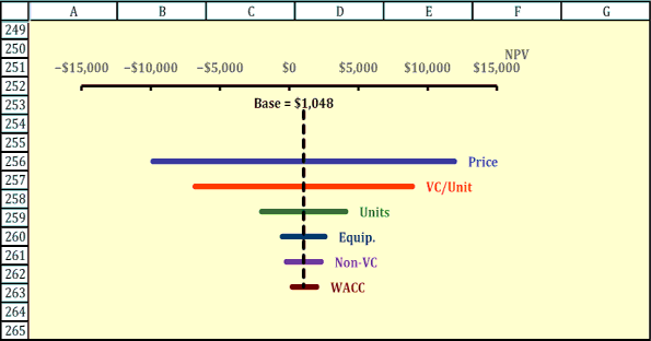
Tornado diagrams are another way to present results from sensitivity analysis. The first steps are to calculate the range of possible for each of the input variables being changed and then rank these ranges. In our example, the range for sales price per unit is the largest and the range for is the smallest. The ranges for each variable are then plotted, with the largest range on top and the smallest range on the bottom. It is also helpful to plot a vertical line showing the base-case NPV. We present a tornado diagram in Figure 11-4. Notice that the diagram is like a tornado in the sense that it is widest at the top and smallest at the bottom; hence its name. The tornado diagram makes it immediately obvious which inputs have the greatest impact on NPV: sales price and variable costs in this case.

Figure 11-4

Tornado Diagram for Solar Water Heater Project: Range of Outcomes for Input Deviations from Base Case (Thousands of Dollars)

11-5c

NPV Break-Even Analysis

Resource

See ch11 Tool Kit.xls on the textbook’s Web site.

A special application of sensitivity analysis is called NPV break-even analysis. In a breakeven analysis, we find the level of an input that produces an of exactly zero. We used Excel’s Goal Seek feature to do this. See ch11 Tool Kit.xls on the textbook’s Web site for an explanation of how to use this Excel feature.

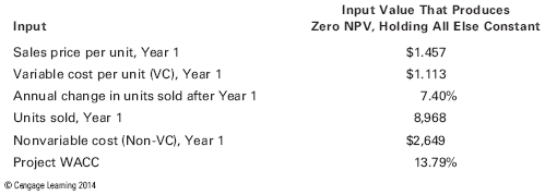
Table 11-1 shows the values of the inputs discussed previously that produce a zero NPV. For example, the number of units sold in Year 1 can drop to before the project’s falls to zero. Break-even analysis is helpful in determining how bad things can get before the project has a negative NPV.

Table 11-1

Break-Even Analysis (Thousands of Dollars)

11-5dExtensions of Sensitivity Analysis

Resource

See ch11 Tool Kit.xlson the textbook’s Web site.

In our examples, we showed how one output, NPV, varied with a change in a single input. Sensitivity analysis can easily be extended to show how multiple outputs, such as  and  , vary with a change in an input. See ch11 Tool Kit.xls on the textbook’s Web site for an example showing how to use Excel’s Data Table feature to present multiple outputs.

It is also possible to use a Data Table to show how a single output, such as NPV, varies for changes in two inputs, such as the number of units sold and the sales price per unit. See ch11 Tool Kit.xls on the textbook’s Web site for an example. However, when we examine the impact of a change in more than one input, we usually use scenario analysis, which is described in the following section.

11-6

Scenario Analysis

In the sensitivity analysis just described, we changed one variable at a time. However, it is useful to know what would happen to the project’s if several of the inputs turn out to be better or worse than expected, and this is what we do in a scenario analysis. Also, scenario analysis allows us to assign probabilities to the base (or most likely) case, the best case, and the worst case; then we can find the expected value and standard deviation of the project’s to get a better idea of the project’s risk.

In a scenario analysis, we begin with the base-case scenario, which uses the most likely value for each input variable. We then ask marketing, engineering, and other operating managers to specify a worst-case scenario (low unit sales, low sales price, high variable costs, and so on) and a best-case scenario. Often, the best and worst cases are defined as having a probability of occurring, with a probability for the base-case conditions. Obviously, conditions could take on many more than three values, but such a scenario setup is useful to help get some idea of the project’s riskiness.

Resource

See ch11 Tool Kit.xls on the textbook’s Web site.

After much discussion with the marketing staff, engineers, accountants, and other experts in the company, a set of worst-case and best-case values were determined for several key inputs. Figure 11-5, taken from worksheet 3a-Scen of the chapter Tool Kit model, shows the probability and inputs assumed for the base-case, worst-case, and best-case scenarios, along with selected key results.

Figure 11-5

Inputs and Key Results for Each Scenario (Thousands of Dollars)

Resource

See ch11 Tool Kit.xls on the textbook’s Web site.

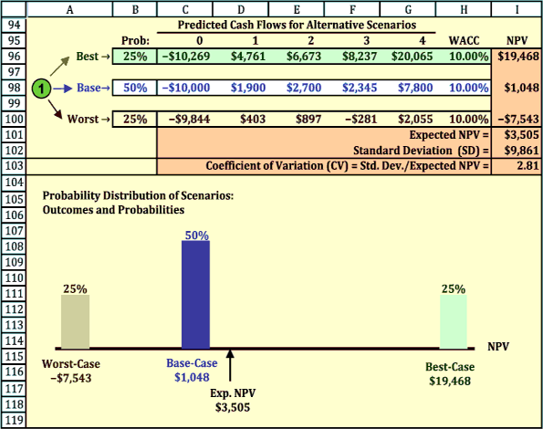
The project’s cash flows and performance measures under each scenario are calculated; see 3a-Scen in the Tool Kit for the calculations. The net cash flows for each scenario are shown in Figure 11-6, along with a probability distribution of the possible outcomes for NPV. If the project is highly successful, then a low initial investment, high sales price, high unit sales, and low production costs would combine to result in a very high NPV, . However, if things turn out badly, then the would be a negative . This wide range of possibilities, and especially the large potential negative value, suggests that this is a risky project. If bad conditions materialize, the project will not bankrupt the company— this is just one project for a large company. Still, losing (actually , as the units are thousands of dollars) would certainly hurt the company’s value and the reputation of the project’s manager.

Figure 11-6

Scenario Analysis: Expected and Its Risk (Thousands of Dollars)

If we multiply each scenario’s probability by the for that scenario and then sum the products, we will have the project’s expected of , as shown in Figure 11-6. Note that the expected differs from the base-case NPV, which is the most likely outcome because it has a probability. This is not an error—mathematically they are not equal. We also calculate the standard deviation of the expected NPV; it is . Dividing the standard deviation by the expected yields the coefficient of variation, , which is a measure of stand-alone risk. The coefficient of variation measures the amount of risk per dollar of NPV, so the coefficient of variation can be helpful when comparing the risk of projects with different . GPC’s average project has a coefficient of variation of about , so the indicates that this project is riskier than most of GPC’s other typical projects.

GPC’s corporate is , so that rate should be used to find the of an average-risk project. However, the water heater project is riskier than average, so a higher discount rate should be used to find its NPV. There is no way to determine the precisely correct discount rate—this is a judgment call. Management decided to evaluate the project using a rate.

Note that the base-case results are the same in our sensitivity and scenario analyses, but in the scenario analysis the worst case is much worse than in the sensitivity analysis and the best case is much better. This is because in scenario analysis all of the variables are set at their best or worst levels, whereas in sensitivity analysis only one variable is adjusted and all the others are left at their base-case levels.

The project has a positive NPV, but its coefficient of variation () is , which is more than double the CV of an average project. With the higher risk, it is not clear if the project should be accepted or not. At this point, GPC’s CEO will ask the CFO to investigate the risk further by performing a simulation analysis, as described in the next section.

11-7

Monte Carlo Simulation

Monte Carlo simulation ties together sensitivities, probability distributions, and correlations among the input variables. It grew out of work in the Manhattan Project to build the first atomic bomb and was so named because it utilized the mathematics of casino gambling. Although Monte Carlo simulation is considerably more complex than scenario analysis, simulation software packages make the process manageable. Many of these packages can be used as add-ins to Excel and other spreadsheet programs.

In a simulation analysis, a probability distribution is assigned to each input variable—sales in units, the sales price, the variable cost per unit, and so on. The computer begins by picking a random value for each variable from its probability distribution. Those values are then entered into the model, the project’s is calculated, and the is stored in the computer’s memory. This is called a trial. After completing the first trial, a second set of input values is selected from the input variables’ probability distributions, and a second is calculated. This process is repeated many times. The from the trials can be charted on a histogram, which shows an estimate of the project’s outcomes. The average of the trials’ is interpreted as a measure of the project’s expected NPV, with the standard deviation (or the coefficient of variation) of the trials’ as a measure of the project’s risk.

Using this procedure, we conducted a simulation analysis of GPC’s solar water heater project. To compare apples and apples, we focused on the same six variables that were allowed to change in the previously conducted scenario analysis. We assumed that each variable can be represented by its own continuous normal distribution with means and standard deviations that are consistent with the base-case scenario. For example, we assumed that the units sold in Year 1 come from a normal distribution with a mean equal to the base-case value of . We used the probabilities and outcomes of the three scenarios from Section 11-6 to estimate the standard deviation (all calculations are in the Tool Kit). The standard deviation of units sold is , as calculated using the scenario values. We made similar assumptions for all variables. In addition, we assumed that the annual change in unit sales will be positively correlated with unit sales in the first year: If demand is higher than expected in the first year, it will continue to be higher than expected. In particular, we assume a correlation of between units sold in the first year and growth in units sold in later years. For all other variables, we assumed zero correlation. Figure 11-7 shows the inputs used in the simulation analysis.

Figure 11-7

Inputs and Key Results for the Current Simulation Trial (Thousands of Dollars)

Figure 11-7 also shows the current set of random variables that were drawn from the distributions at the time we created the figure for the textbook—you will see different values for the key results when you look at the Excel model because the values are updated every time the file is opened. We used a two-step procedure to create the random variables for the inputs. First, we used Excel’s functions to generate standard normal random variables with a mean of and a standard deviation of ; these are shown in Cells E38: E51. To create the random values for the inputs used in the analysis, we multiplied a random standard normal variable by the standard deviation and added the expected value. For example, Excel drew the value for first-year unit sales (Cell E42) from a standard normal distribution. We calculated the value for first-year unit sales to use in the current trial as , which is shown in Cell F42.

We used the inputs in Cells F38:F52 to generate cash flows and to calculate performance measures for the project (the calculations are in the Tool Kit). For the trial reported in Figure 11-7, the is . We used a Data Table in the Tool Kit to generate additional trials. For each trial, the Data Table saved the value of the input variables and the value of the trial’s NPV. Figure 11-8 presents selected results from the simulation for trials. (The worksheet 4a-Sim100 in the Tool Kit shows only trials; the worksheet 4b-Sim10000 has the ability to perform simulations, but we have turned off the Data Table in that worksheet because simulating trials reduces Excel’s speed when performing other calculations in the file.)

Resource

See ch11 Tool Kit.xls on the textbook’s Web site.

After running a simulation, the first thing we do is verify that the results are consistent with our assumptions. The resulting sample mean and standard deviation of units sold in the first year are and , which are virtually identical to our assumptions in Figure 11-7. The same is true for all the other inputs, so we can be reasonably confident that the simulation is doing what we are asking. Figure 11-8 also reports summary statistics for the project’s NPV. The mean is , which suggests that the project should be accepted. However, the range of outcomes is quite large, from a loss of to a gain of , so the project is clearly risky. The standard deviation of indicates that losses could easily occur, which is consistent with this wide range of possible outcomes.Figure 11-8 also reports a median of , which means that half the time the project will have an of less than . In fact, there is only probability that the project will have a positive .

Figure 11-8

Summary of Simulation Results (Thousands of Dollars)

A picture is worth a thousand words, and Figure 11-8 shows the probability distribution of the outcomes. Note that the distribution of outcomes is slightly skewed to the right. As the figure shows, the potential downside losses are not as large as the potential upside gains. Our conclusion is that this is a very risky project, as indicated by the coefficient of variation, but it does have a positive expected and the potential to be a “home run.”

Resource

See ch11 Tool Kit.xls on the textbook’s Web site.

If the company decides to go ahead with the project, senior management should also identify possible contingency plans for responding to changes in market conditions. Senior managers always should consider qualitative factors in addition to the quantitative project analysis.

We have discussed the three types of risk normally considered in capital budgeting: stand alone risk, within-firm (or corporate) risk, and market risk. However, two important questions remain: 

• (1)

Should firms care about stand-alone and corporate risk, given that finance theory says that market (beta) risk is the only relevant risk?

• (2)

What do we do when the stand-alone, within-firm, and market risk assessments lead to different conclusions?

There are no easy answers to these questions. Strict adherents of the CAPM would argue that well-diversified investors are concerned only with market risk, that managers should be concerned only with maximizing stock price, and thus that market (beta) risk ought to be given virtually all the weight in capital budgeting decisions. However, we know that not all investors are well diversified, that the CAPM does not operate exactly as the theory says it should, and that measurement problems keep managers from having complete confidence in the CAPM inputs. In addition, the CAPM ignores bankruptcy costs, even though such costs can be substantial, and the probability of bankruptcy depends on a firm’s corporate risk, not on its beta risk. Therefore, even well-diversified investors should want a firm’s management to give at least some consideration to a project’s corporate risk, and that means giving some consideration to stand-alone project risk.

Although it would be nice to reconcile these problems and to measure risk on some absolute scale, the best we can do in practice is to estimate risk in a somewhat nebulous, relative sense. For example, we can generally say with a fair degree of confidence that a particular project has more, less, or about the same stand-alone risk as the firm’s average project. Then, because stand-alone and corporate risks generally are correlated, the project’s stand-alone risk generally is a reasonably good measure of its corporate risk. Finally, assuming that market risk and corporate risk are correlated, as is true for most companies, a project with a relatively high or low corporate risk will also have a relatively high or low market risk. We wish we could be more specific, but one simply must use a lot of judgment when assessing projects’ risks.

According to traditional capital budgeting theory, a project’s  is the present value of its expected future cash flows discounted at a rate that reflects the riskiness of those cash flows. Note, however, that this says nothing about actions taken after the project has been accepted and placed in operation that might lead to an increase in the cash flows. In other words, traditional capital budgeting theory assumes that a project is like a roulette wheel. A gambler can choose whether to spin the wheel, but once the wheel has been spun, nothing can be done to influence the outcome. Once the game begins, the outcome depends purely on chance, and no skill is involved.

Contrast roulette with a game such as poker. Chance plays a role in poker, and it continues to play a role after the initial deal because players receive additional cards throughout the game. However, poker players are able to respond to their opponents’ actions, so skilled players usually win.

Capital budgeting decisions have more in common with poker than roulette because 

• (1)

chance plays a continuing role throughout the life of the project, but

• (2)

managers can respond to changing market conditions and to competitors’ actions.

Opportunities to respond to changing circumstances are called managerial options(because they give managers a chance to influence the outcome of a project), strategic options (because they are often associated with large, strategic projects rather than routine maintenance projects), and embedded options (because they are a part of the project). Finally, they are called real options to differentiate them from financial options because they involve real, rather than financial, assets. The following sections describe projects with several types of real options.

Conventional  analysis implicitly assumes that projects either will be accepted or rejected, which implies they will be undertaken now or never. In practice, however, companies sometimes have a third choice—delay the decision until later, when more information is available. Such investment timing options can dramatically affect a project’s estimated profitability and risk, as we saw in our example of GPC’s solar water heater project.

Keep in mind, though, that the option to delay is valuable only if it more than offsets any harm that might result from delaying. For example, while one company delays, some other company might establish a loyal customer base that makes it difficult for the first company to enter the market later. The option to delay is usually most valuable to firms with proprietary technology, patents, licenses, or other barriers to entry, because these factors lessen the threat of competition. The option to delay is valuable when market demand is uncertain, but it is also valuable during periods of volatile interest rates, because the ability to wait can allow firms to delay raising capital for a project until interest rates are lower.

A growth option allows a company to increase its capacity if market conditions are better than expected. There are several types of growth options. One lets a company increase the capacity of an existing product line. A “peaking unit” power plant illustrates this type of growth option. Such units have high variable costs and are used to produce additional power only if demand, thus prices, are high.

The second type of growth option allows a company to expand into new geographic markets. Many companies are investing in China, Eastern Europe, and Russia even though standard  analysis produces negative  . However, if these developing markets really take off, the option to open more facilities could be quite valuable.

The third type of growth option is the opportunity to add new products, including complementary products and successive “generations” of the original product. Auto companies are losing money on their first electric autos, but the manufacturing skills and consumer recognition those cars will provide should help turn subsequent generations of electric autos into moneymakers.

Consider the value of an abandonment option. Standard DCF analysis assumes that a project’s assets will be used over a specified economic life. But even though some projects must be operated over their full economic life—in spite of deteriorating market conditions and hence lower than expected cash flows—other projects can be abandoned. Smart managers negotiate the right to abandon if a project turns out to be unsuccessful as a condition for undertaking the project.

Note, too, that some projects can be structured so that they provide the option to reduce capacity or temporarily suspend operations. Such options are common in the natural resources industry, including mining, oil, and timber, and they should be reflected in the analysis when  are being estimated.

Many projects offer flexibility options that permit the firm to alter operations depending on hed. BMW’s Spartanburg, South Carolina, auto assembly plant provides a good example of output flexibility. BMW needed the plant to produce sports coupes. If it built the plant configured to produce only these vehicles, the construction cost would be minimized. However, the company thought that later on it might want to switch production to some other vehicle type, and that would be difficult if the plant were designed just for coupes. Therefore, BMW decided to spend additional funds to construct a more flexible plant: one that could produce different types of vehicles should demand patterns shift. Sure enough, things did change. Demand for coupes dropped a bit and demand for sport-utility vehicles soared. But BMW was ready, and the Spartanburg plant began to produce hot-selling SUVs. The plant’s cash flows were much higher than they would have been without the flexibility option that BMW “bought” by paying more to build a more flexible plant.

Electric power plants provide an example of input flexibility. Utilities can build plants that generate electricity by burning coal, oil, or natural gas. The prices of those fuels change over time in response to events in the Middle East, changing environmental policies, and weather conditions. Some years ago, virtually all power plants were designed to burn just one type of fuel, because this resulted in the lowest construction costs. However, as fuel cost volatility increased, power companies began to build higher-cost but more flexible plants, especially ones that could switch from oil to gas and back again depending on relative fuel prices.

A full treatment of real option valuation is beyond the scope of this chapter, but there are some things we can say. First, if a project has an embedded real option, then management should at least recognize and articulate its existence. Second, we know that a financial option is more valuable if it has a long time until maturity or if the underlying asset is very risky. If either of these characteristics applies to a project’s real option, then management should know that its value is probably relatively high. Third, management might be able to model the real option along the lines of a decision tree, as we illustrate in the following section.

Up to this point we have focused primarily on techniques for estimating a project’s risk. Although this is an integral part of capital budgeting, managers are just as interested in reducing risk as in measuring it. One way to reduce risk is to structure projects so that expenditures can be made in stages over time rather than all at once. This gives managers the opportunity to reevaluate decisions using new information and then to either invest additional funds or terminate the project. This type of analysis involves the use of decision trees.

11-11a

The Basic Decision Tree

Resource

See ch11 Tool Kit.xls on the textbook’s Web site.

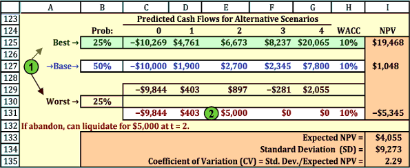
GPC’s analysis of the solar water heater project thus far has assumed that the project cannot be abandoned once it goes into operation, even if the worst-case situation arises. However, GPC is considering the possibility of terminating (abandoning) the project at Year 2 if the demand is low. The net after-tax cash flow from salvage, legal fees, liquidation of working capital, and all other termination costs and revenues is . Using these assumptions, the GPC ran a new scenario analysis; the results are shown in Figure 11-10, which is a simple decision tree.

Figure 11-10

Simple Decision Tree: Abandoning Project in Worst-Case Scenario

Here we assume that, if the worst case materializes, then this will be recognized after the low Year-1 cash flow and GPC will abandon the project. Rather than continue realizing low cash flows in Years 2, 3, and 4, the company will shut down the operation and liquidate the project for at . Now the expected rises from to and the CV declines from to . So, securing the right to abandon the project if things don’t work out raised the project’s expected return and lowered its risk. This will give you an approximate value, but keep in mind that you may not have a good estimate of the appropriate discount rate because the real option changes the risk, and hence the required return, of the project.

11-11b

Staged Decision Tree

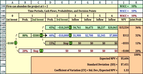
After the management team thought about the decision-tree approach, other ideas for improving the project emerged. The marketing manager stated that he could undertake a study that would give the firm a better idea of demand for the product. If the marketing study found favorable responses to the product, the design engineer stated that she could build a prototype solar water heater to gauge consumer reactions to the actual product. After assessing consumer reactions, the company could either go ahead with the project or abandon it. This type of evaluation process is called a staged decision tree and is shown in Figure 11-11.

Figure 11-11

Decision Tree with Multiple Decision Points

Decision trees such as the one in Figure 11-11 often are used to analyze multistage, or sequential, decisions. Each circle represents a decision point, also known as a decision node. The dollar value to the left of each decision node represents the net cash flow at that point, and the cash flows shown under , , , and represent the cash inflows if the project is pushed on to completion. Each diagonal line leads to a branch of the decision tree, and each branch has an estimated probability. For example, if the firm decides to “go” with the project at Decision Point 1, then it will spend on the marketing study. Management estimates that there is a probability that the study will produce positive results, leading to the decision to make an additional investment and thus move on to Decision Point 2, and a probability that the marketing study will produce negative results, indicating that the project should be canceled after Stage 1. If the project is canceled, the cost to the company will be the spent on the initial marketing study.

If the marketing study yields positive results, then the firm will spend on the prototype water heater module at Decision Point 2. Management estimates (even before making the initial investment) that there is a probability of the pilot project yielding good results, a probability of average results, and a probability of bad results. If the prototype works well, then the firm will spend several millions more at Decision Point 3 to build a production plant, buy the necessary inventory, and commence operations. The operating cash flows over the project’s life will be good, average, or bad, and these cash flows are shown under Years 3 through 6.

The column of joint probabilities in Figure 11-11 gives the probability of occurrence of each branch—and hence of each NPV. Each joint probability is obtained by multiplying together all the probabilities on that particular branch. For example, the probability that the company will, if Stage 1 is undertaken, move through Stages 2 and 3, and that a strong demand will produce the indicated cash flows, is . There is a probability of average results, a probability of building the plant and then getting bad results, and a probability of getting bad initial results and stopping after the marketing study. The of the top (most favorable) branch as shown in Column J is , calculated as follows:

The for the other branches are calculated similarly.

The last column in Figure 11-11 gives the product of the for each branch times the joint probability of that branch’s occurring, and the sum of these products is the project’s expected NPV. Based on the expectations used to create Figure 11-11 and a cost of capital of , the project’s expected is , or . In addition, the CV declines from to , and the maximum anticipated loss is a manageable . At this point, the solar water heater project looked good, and GPC’s management decided to accept it.

As this example shows, decision-tree analysis requires managers to articulate explicitly the types of risk a project faces and to develop responses to potential scenarios. Note also that our example could be extended to cover many other types of decisions and could even be incorporated into a simulation analysis. All in all, decision-tree analysis is a valuable tool for analyzing project risks.