Based on the text on regression assumptions and your additional research, discuss the potential impact of assumption violation on interpretation of regression results. Is there any influence of the assumption violation on the business decision making? If
The future is uncertain. Some events do have a very small probability of happening, like an asteroid destroying the earth. So we accept that tomorrow will come as a certain event. But future demand for a business’s goods and services is very uncertain. Yet, the management of a company wants to have some idea of the survival (or growth) of the company in the future. Should they expect to hire more people or let some go? Should they plan to increase capacity? How much investment is needed for future assets, or should they down size?
Forecasting provides some ideas about the future, but how this is accomplished can vary from company to company. And one key factor is how accurate the forecast is. Generally, the further into the future one looks, the more uncertain the information is. How do forecasters reduce their forecasting errors? How much error is tolerable?
Another key factor in forecasting is data availability. Data processing and storage capability have become extremely available and inexpensive. Software and computing power is also very cheap. Collecting real-time sales data via point-of-sales systems is now common at most retail establishments. But couple this with a situation in companies that have a large number of products, such as a retail store or a large manufacturing company with hundreds or thousands of product numbers and/or product lines, forecasting becomes complicated.
Forecasting Methods
There are two main types or genres of forecasting methods, qualitative and quantitative. The former consists of judgment and analysis of qualitative factors, such as scenario building and scenario analysis. The latter is obviously based on numerical analysis. This genre of forecasting includes such methods as linear regression, time series analysis, and data mining algorithms like CHAID and CART, which are useful especially in the growing world of artificial intelligence and machine learning in business. This module will look at the linear regression and time series analysis using exponential smoothing.
Linear Growth
When using any mathematical model, we have to consider which inputs are reasonable to use. Whenever we extrapolate, or make predictions into the future, we are assuming the model will continue to be valid. There are different types of mathematical model, one of which is linear growth model or algebraic growth model and another is exponential growth model, or geometric growth model. The constant change is the defining characteristic of linear growth. Plotting the values, we can see the values form a straight line, the shape of linear growth.
If a quantity starts at size P0 and grows by d every time period, then the quantity after n time periods can be determined using either of these relations:
Recursive form:
Pn = Pn-1 + d
Explicit form:
Pn = P0 + d n
In this equation, d represents the common difference – the amount that the population changes each time n increases by 1. Calculating values using the explicit form and plotting them with the original data shows how well our model fits the data. We can now use our model to make predictions about the future, assuming that the previous trend continues unchanged.
Exponential Growth
If a quantity starts at size P0 and grows by R% (written as a decimal, r) every time period, then the quantity after n time periods can be determined using either of these relations:
Recursive form:
Pn = (1+r) Pn-1
Explicit form:
Pn = (1+r)n P0 or equivalently, Pn = P0 (1+r)n
We call r the growth rate and the term (1+r) is called the growth multiplier, or common ratio.
In exponential growth, the population grows proportional to the size of the population, so as the population gets larger, the same percent growth will yield a larger numeric growth.
Linear regression is a very powerful statistical technique. Many people have some familiarity with regression just from reading the news, where graphs with straight lines are overlaid on scatterplots. Linear models can be used for prediction or to evaluate whether there is a linear relationship between two numerical variables.
Figure 1 shows two variables whose relationship can be modeled perfectly with a straight line. The equation for the line is
y=5+57.49x
Imagine what a perfect linear relationship would mean: you would know the exact value of y just by knowing the value of x. This is unrealistic in almost any natural process. For example, if we took family income x, this value would provide some useful information about how much financial support y a college may offer a prospective student. However, there would still be variability in financial support, even when comparing students whose families have similar financial backgrounds.
Linear regression assumes that the relationship between two variables, x and y, can be modeled by a straight line:
β0+β1xβ0+β1x
where β0 and β1 represent two model parameters (β is the Greek letter beta). These parameters are estimated using data, and we write their point estimates as b0 and b1. When we use x to predict y, we usually call x the explanatory or predictor or independent variable, and we call y the response or dependent variable.
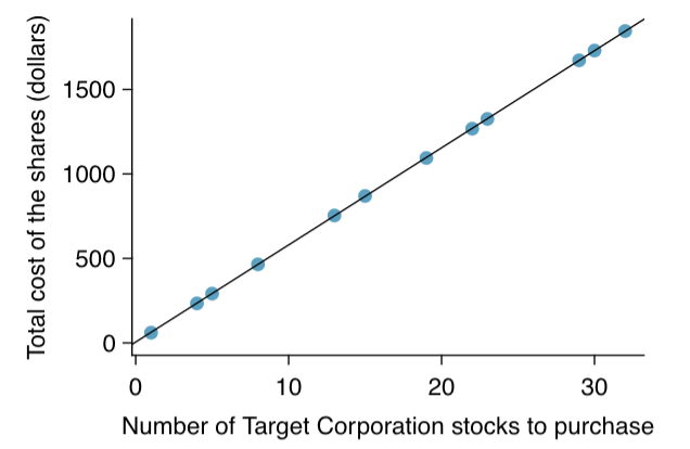
Figure 1
Figure 1 shows that requests from twelve separate buyers were simultaneously placed with a trading company to purchase Target Corporation stock (ticker TGT, April 26th, 2012), and the total cost of the shares were reported. Because the cost is computed using a linear formula, the linear fit is perfect.
It is rare for all of the data to fall on a straight line, as seen in the three scatterplots in Figure 2. In each case, the data fall around a straight line, even if none of the observations fall exactly on the line. The first plot shows a relatively strong downward linear trend, where the remaining variability in the data around the line is minor relative to the strength of the relationship between x and y. The second plot shows an upward trend that, while evident, is not as strong as the first. The last plot shows a very weak downward trend in the data, so slight we can hardly notice it. In each of these examples, we will have some uncertainty regarding our estimates of the model parameters, β0 and β1. For instance, we might wonder, should we move the line up or down a little, or should we tilt it more or less?
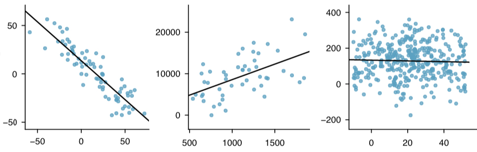
Figure 2
Figure 2 shows the three data sets where a linear model may be useful even though the data do not all fall exactly on the line. As we move forward in this module, we will learn different criteria for line-fitting, and we will also learn about the uncertainty associated with estimates of model parameters. We will also see examples where fitting a straight line to the data, even if there is a clear relationship between the variables, is not helpful. One such case is shown in Figure 3 where there is a very strong relationship between the variables even though the trend is not linear.
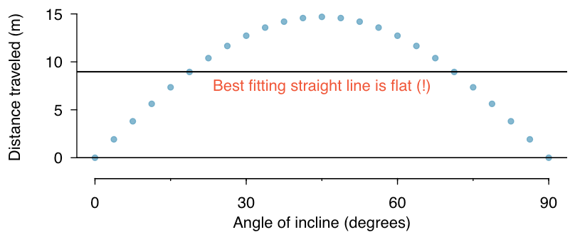
Figure 3. A linear model is not useful in this nonlinear case. These data are from an introductory physics experiment.
Simple Linear Regression vs. Multiple Regression
In simple linear regression, a criterion variable or dependent variable is predicted from one predictor variable. In multiple regression, the criterion is predicted by two or more independent or predictor variables. Take the SAT case study for an example, you might want to predict a student's university grade point average on the basis of their High-School GPA (HSGPA) and their total SAT score (verbal + math). The basic idea is to find a linear combination of HSGPA and SAT that best predicts University GPA (UGPA). That is, the problem is to find the values of b1 and b2 in the equation shown below that give the best predictions of UGPA. As in the case of simple linear regression, we define the best predictions as the predictions that minimize the squared errors of prediction.
UGPA' = b1HSGPA + b2SAT + A
where UGPA' is the predicted value of University GPA and A is a constant. For these data, the best prediction equation is shown below:
UGPA' = 0.541 x HSGPA + 0.008 x SAT + 0.540
In other words, to compute the prediction of a student's University GPA, you add up (a) their High-School GPA multiplied by 0.541, (b) their SAT multiplied by 0.008, and (c) 0.540. Table 1 shows the data and predictions for the first five students in the dataset.
Table 1. Data and Predictions.
| HSGPA | SAT | UGPA' |
| 3.45 | 1232 | 3.38 |
| 2.78 | 1070 | 2.89 |
| 2.52 | 1086 | 2.76 |
| 3.67 | 1287 | 3.55 |
| 3.24 | 1130 | 3.19 |
The values of b (b1 and b2) are sometimes called "regression coefficients" and sometimes called "regression weights." These two terms are synonymous. The multiple correlation (R) is equal to the correlation between the predicted scores and the actual scores. In this example, it is the correlation between UGPA' and UGPA, which turns out to be 0.79. That is, R = 0.79. Note that R will never be negative since if there are negative correlations between the predictor variables and the criterion, the regression weights will be negative so that the correlation between the predicted and actual scores will be positive.
Interpretation of Regression Coefficients
A regression coefficient in multiple regression is the slope of the linear relationship between the criterion variable and the part of a predictor variable that is independent of all other predictor variables. In this example, the regression coefficient for HSGPA can be computed by first predicting HSGPA from SAT and saving the errors of prediction (the differences between HSGPA and HSGPA'). These errors of prediction are called "residuals" since they are what is left over in HSGPA after the predictions from SAT are subtracted, and represent the part of HSGPA that is independent of SAT. These residuals are referred to as HSGPA.SAT, which means they are the residuals in HSGPA after having been predicted by SAT. The correlation between HSGPA.SAT and SAT is necessarily 0.
The final step in computing the regression coefficient is to find the slope of the relationship between these residuals and UGPA. This slope is the regression coefficient for HSGPA. The following equation is used to predict HSGPA from SAT:
HSGPA' = -1.314 + 0.0036 x SAT
The residuals are then computed as:
HSGPA - HSGPA'
The linear regression equation for the prediction of UGPA by the residuals is
UGPA' = 0.541 x HSGPA.SAT + 3.173
Notice that the slope (0.541) is the same value given previously for b1 in the multiple regression equation.
This means that the regression coefficient for HSGPA is the slope of the relationship between the criterion variable and the part of HSGPA that is independent of (uncorrelated with) the other predictor variables. It represents the change in the criterion variable associated with a change of one in the predictor variable when all other predictor variables are held constant. Since the regression coefficient for HSGPA is 0.54, this means that, holding SAT constant, a change of one in HSGPA is associated with a change of 0.54 in UGPA'. If two students had the same SAT and differed in HSGPA by 2, then you would predict they would differ in UGPA by (2)(0.54) = 1.08. Similarly, if they differed by 0.5, then you would predict they would differ by (0.50)(0.54) = 0.27.
The slope of the relationship between the part of a predictor variable independent of other predictor variables and the criterion is its partial slope. Thus the regression coefficient of 0.541 for HSGPA and the regression coefficient of 0.008 for SAT are partial slopes. Each partial slope represents the relationship between the predictor variable and the criterion holding constant all of the other predictor variables.
It is difficult to compare the coefficients for different variables directly because they are measured on different scales. A difference of 1 in HSGPA is a fairly large difference, whereas a difference of 1 on the SAT is negligible. Therefore, it can be advantageous to transform the variables so that they are on the same scale. The most straightforward approach is to standardize the variables so that they each have a standard deviation of 1. A regression weight for standardized variables is called a "beta weight" and is designated by the Greek letter β. For these data, the beta weights are 0.625 and 0.198. These values represent the change in the criterion (in standard deviations) associated with a change of one standard deviation on a predictor [holding constant the value(s) on the other predictor(s)]. Clearly, a change of one standard deviation on HSGPA is associated with a larger difference than a change of one standard deviation of SAT. In practical terms, this means that if you know a student's HSGPA, knowing the student's SAT does not aid the prediction of UGPA much. However, if you do not know the student's HSGPA, his or her SAT can aid in the prediction since the β weight in the simple regression predicting UGPA from SAT is 0.68. For comparison purposes, the β weight in the simple regression predicting UGPA from HSGPA is 0.78. As is typically the case, the partial slopes are smaller than the slopes in simple regression.
Partitioning the Sums of Squares
Just as in the case of simple linear regression, the sum of squares for the criterion (UGPA in this example) can be partitioned into the sum of squares predicted and the sum of squares error. That is,
SSY = SSY' + SSE
which for these data:
20.798 = 12.961 + 7.837
The sum of squares predicted is also referred to as the "sum of squares explained." Again, as in the case of simple regression,
Proportion Explained = SSY'/SSY
In simple regression, the proportion of variance explained is equal to r2; in multiple regression, the proportion of variance explained is equal to R2. In multiple regression, it is often informative to partition the sum of squares explained among the predictor variables. For example, the sum of squares explained for these data is 12.96. How is this value divided between HSGPA and SAT?
One approach that, as will be seen, does not work is to predict UGPA in separate simple regressions for HSGPA and SAT. As can be seen in Table 2, the sum of squares in these separate simple regressions is 12.64 for HSGPA and 9.75 for SAT. If we add these two sums of squares we get 22.39, a value much larger than the sum of squares explained of 12.96 in the multiple regression analysis. The explanation is that HSGPA and SAT are highly correlated (r = .78) and therefore much of the variance in UGPA is confounded between HSGPA and SAT. That is, it could be explained by either HSGPA or SAT and is counted twice if the sums of squares for HSGPA and SAT are simply added.
Table 2. Sums of Squares for Various Predictors
| Predictors | Sum of Squares |
| HSGPA | 12.64 |
| SAT | 9.75 |
| HSGPA and SAT | 12.96 |
Table 3 shows the partitioning of the sum of squares into the sum of squares uniquely explained by each predictor variable, the sum of squares confounded between the two predictor variables, and the sum of squares error. It is clear from this table that most of the sum of squares explained is confounded between HSGPA and SAT. Note that the sum of squares uniquely explained by a predictor variable is analogous to the partial slope of the variable in that both involve the relationship between the variable and the criterion with the other variable(s) controlled.
Table 3. Partitioning the Sum of Squares
| Source | Sum of Squares | Porportion |
| HSGPA (unique) | 3.21 | 0.15 |
| SAT (unique) | 0.32 | 0.02 |
| HSGPA and SAT (Confounded) | 9.43 | 0.45 |
| Error | 7.84 | 0.38 |
| Total | 20.80 | 1.00 |
The sum of squares uniquely attributable to a variable is computed by comparing two regression models: the complete model and a reduced model. The complete model is the multiple regression with all the predictor variables included (HSGPA and SAT in this example). A reduced model is a model that leaves out one of the predictor variables. The sum of squares uniquely attributable to a variable is the sum of squares for the complete model minus the sum of squares for the reduced model in which the variable of interest is omitted. As shown in Table 2, the sum of squares for the complete model (HSGPA and SAT) is 12.96. The sum of squares for the reduced model in which HSGPA is omitted is simply the sum of squares explained using SAT as the predictor variable and is 9.75. Therefore, the sum of squares uniquely attributable to HSGPA is 12.96 - 9.75 = 3.21. Similarly, the sum of squares uniquely attributable to SAT is 12.96 - 12.64 = 0.32. The confounded sum of squares in this example is computed by subtracting the sum of squares uniquely attributable to the predictor variables from the sum of squares for the complete model: 12.96 - 3.21 - 0.32 = 9.43. The computation of the confounded sums of squares in analyses with more than two predictors is more complex and beyond the scope of this text.
Since the variance is simply the sum of squares divided by the degrees of freedom, it is possible to refer to the proportion of variance explained in the same way as the proportion of the sum of squares explained. It is slightly more common to refer to the proportion of variance explained than the proportion of the sum of squares explained. When variables are highly correlated, the variance explained uniquely by the individual variables can be small even though the variance explained by the variables taken together is large. For example, although the proportions of variance explained uniquely by HSGPA and SAT are only 0.15 and 0.02 respectively, together these two variables explain 0.62 of the variance. Therefore, you could easily underestimate the importance of variables if only the variance explained uniquely by each variable is considered. Consequently, it is often useful to consider a set of related variables. For example, assume you were interested in predicting job performance from a large number of variables some of which reflect cognitive ability. It is likely that these measures of cognitive ability would be highly correlated among themselves and therefore no one of them would explain much of the variance independently of the other variables. However, you could avoid this problem by determining the proportion of variance explained by all of the cognitive ability variables considered together as a set. The variance explained by the set would include all the variance explained uniquely by the variables in the set as well as all the variance confounded among variables in the set. It would not include variance confounded with variables outside the set. In short, you would be computing the variance explained by the set of variables that is independent of the variables not in the dataset.
Inferential Statistics
We begin by presenting the formula for testing the significance of the contribution of a set of variables. We will then show how special cases of this formula can be used to test the significance of R2 as well as to test the significance of the unique contribution of individual variables.
The first step is to compute two regression analyses: (1) an analysis in which all the predictor variables are included and (2) an analysis in which the variables in the set of variables being tested are excluded. The former regression model is called the "complete model" and the latter is called the "reduced model." The basic idea is that if the reduced model explains much less than the complete model, then the set of variables excluded from the reduced model is important.
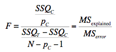
The formula for testing the contribution of a group of variables is:
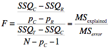
where:
SSQC is the sum of squares for the complete model,
SSQR is the sum of squares for the reduced model,
pC is the number of predictors in the complete model,
pR is the number of predictors in the reduced model,
SSQT is the sum of squares total (the sum of squared deviations of the criterion variable from its mean), and
N is the total number of observations
The degrees of freedom for the numerator is pC - pR and the degrees of freedom for the denominator is N - pc -1. If the F is significant, then it can be concluded that the variables excluded in the reduced set contribute to the prediction of the criterion variable independently of the other variables. This formula can be used to test the significance of R2 by defining the reduced model as having no predictor variables. In this application, SSQR and pR = 0. The formula is then simplified as follows:
which for this example becomes:
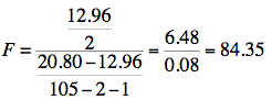
The degrees of freedom are 2 and 102. The F distribution calculator shows that p < 0.001.
F Calculator
The reduced model used to test the variance explained uniquely by a single predictor consists of all the variables except the predictor variable in question. For example, the reduced model for a test of the unique contribution of HSGPA contains only the variable SAT. Therefore, the sum of squares for the reduced model is the sum of squares when UGPA is predicted by SAT. This sum of squares is 9.75. The calculations for F are shown below:
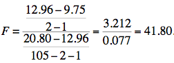
The degrees of freedom are 1 and 102. The F distribution calculator shows that p < 0.001.
Similarly, the reduced model in the test for the unique contribution of SAT consists of HSGPA.
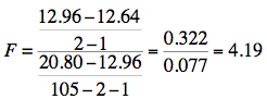
The degrees of freedom are 1 and 102. The F distribution calculator shows that p = 0.0432.
The significance test of the variance explained uniquely by a variable is identical to a significance test of the regression coefficient for that variable. A regression coefficient and the variance explained uniquely by a variable both reflect the relationship between a variable and the criterion independent of the other variables. If the variance explained uniquely by a variable is not zero, then the regression coefficient cannot be zero. Clearly, a variable with a regression coefficient of zero would explain no variance.
Other inferential statistics associated with multiple regression are beyond the scope of this text. Two of particular importance are (1) confidence intervals on regression slopes and (2) confidence intervals on predictions for specific observations. These inferential statistics can be computed by standard statistical analysis packages such as R, SPSS, STATA, SAS, and JMP.
Assumptions
No assumptions are necessary for computing the regression coefficients or for partitioning the sum of squares. However, there are several assumptions made when interpreting inferential statistics. Moderate violations of Assumptions 1-3 do not pose a serious problem for testing the significance of predictor variables. However, even small violations of these assumptions pose problems for confidence intervals on predictions for specific observations.
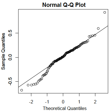
Residuals are normally distributed:
As in the case of simple linear regression, the residuals are the errors of prediction. Specifically, they are the differences between the actual scores on the criterion and the predicted scores. A Q-Q plot for the residuals for the example data is shown below. This plot reveals that the actual data values at the lower end of the distribution do not increase as much as would be expected for a normal distribution. It also reveals that the highest value in the data is higher than would be expected for the highest value in a sample of this size from a normal distribution. Nonetheless, the distribution does not deviate greatly from normality.
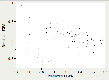
Homoscedasticity:
It is assumed that the variances of the errors of prediction are the same for all predicted values. As can be seen below, this assumption is violated in the example data because the errors of prediction are much larger for observations with low-to-medium predicted scores than for observations with high predicted scores. Clearly, a confidence interval on a low predicted UGPA would underestimate the uncertainty.
Linearity:
It is assumed that the relationship between each predictor variable and the criterion variable is linear. If this assumption is not met, then the predictions may systematically overestimate the actual values for one range of values on a predictor variable and underestimate them for another.
Time Series Analysis and Exponential Smoothing Forecasting
In this Module you will also learn another forecasting model, time series analysis. We may not have a causal relationship that we can use. In this situation we must use the time series data by itself. We may have daily, weekly, monthly or quarterly data of demand, sales, or another factor we need to forecast. The main assumption is that the best forecast of the next period is based on the previous demand values with some adjustment. The question is how much weight should be given to the recent data and older data. The Moving Average method is a simple technique. And an even simpler method to implement is the Exponential Smoothing technique.
Time series graphs are important tools in various applications of statistics. When recording values of the same variable over an extended period of time, sometimes it is difficult to discern any trend or pattern. However, once the same data points are displayed graphically, some features jump out. Time series graphs make trends easy to spot.
We can start with a standard Cartesian coordinate system. The horizontal axis is used to plot the date or time increments, and the vertical axis is used to plot the values of the variable that we are measuring. By doing this, we make each point on the graph correspond to a date and a measured quantity. The points on the graph are typically connected by straight lines in the order in which they occur.
Download the Excel file Module 2 SLP Practice Example that contains an example and a Practice Exercise. Watch this video that shows how to do SES and calculate MAPE: http://permalink.fliqz.com/aspx/permalink.aspx?at=75d6cc75bbe742159e56ad8836531c1d&a=5fae3cf0f1624f39b0341263a6541ea0
PRACTICE: Download the Excel file Module 2 Case Practice Example which provides an examples and practice problems to learn how to do regression analysis in Excel.
Licenses and Attributions
Online Statistics Education: A Multimedia Course of Study (http://onlinestatbook.com/). Project Leader: David M. Lane, Rice University.
CC licensed content, Shared previously
OpenStax, Statistics, Histograms, Frequency Polygons, and Time Series Graphs. Provided by: OpenStax. Located at: http://cnx.org/contents/[email protected]:11/Introductory_Statistics. License: CC BY: Attribution
Math in Society. Authored by: Open Textbook Store, Transition Math Project, and the Open Course Library. Located at: http://www.opentextbookstore.com/mathinsociety/. License: CC BY-SA: Attribution-ShareAlike
OpenIntro Statistics. Authored by: David M Diez, Christopher D Barr, and Mine Cetinkaya-Rundel. Provided by: OpenIntro. Located at: https://www.openintro.org/stat/textbook.php. License: CC BY-SA: Attribution-ShareAlike. License Terms: This textbook is available under a Creative Commons license. Visit openintro.org for a free PDF, to download the textbook's source files.
Optional Reading
Chase, C. W., (2013). Demand-driven forecasting: A structured approach to forecasting. John Wiley & Sons. Somerset, NJ. Retrieved from Ebrary in the Trident Online Library.
Check the following chapters of Chase (2013):
Chapter 3, pp. 91–93 (the section Some Causes of Forecast Error)
Chapter 4, pp. 103–113, which provides information on forecast error measures; pay special attention to the sections on the MAPE measurement
Chapter 5, pp. 125–147; pay attention the sections on Simple Exponential Smoothing (SES)
Two videos on Khan Academy showing how to calculate regression coefficients:
Regression Line Example: http://www.khanacademy.org/video/regression-line-example?topic=statistics
Second Regression Example: http://www.khanacademy.org/video/second-regression-example?topic=statistics


