Policy analysis: Prescribing policies

PRESCRIBING POLICIES

Week 7 Assignment #3

Joseph Brown

Dr. Richard Freeman

PAD-520

June 23rd, 2013

Determine the following before deciding a prescription: (a) maximize effectiveness at the least cost; (b) maximize effectiveness at a fixed cost of $10,000; (c) achieve a fixed-effectiveness level of 6,000 units of service at a fixed cost of $20,000; (d) maximize net benefits, assuming that each unit of service has a market price of $10; (e) maximize the ration of benefits to costs, assuming that each unit of service has a market price of $10.

In order to determine the following, an adequacy method must be applied. “Adequacy refers to the extent to which any given level of effectiveness satisfies a particular standard. The criterion of adequacy specifies expectations about the strength of a relationship between policy alternatives and a fixed or variable value of a desired outcome’ (Dunn 2012, Pp., 197). The following can be determining as: (a) maximize effectiveness at the least cost is a Type II problem. (b) Maximize effectiveness at a fixed cost of $10,000 is a Type I problem. (c) Achieve a fixed-effectiveness level of 6,000 units of services at a fixed cost of $20,000 is a Type II problem. (d) Maximize net benefits, assuming that each unit of service has a market price of $10 is a Type I problem. (e) Maximize the ration of benefits to costs; assuming that each unit of service has a market price of $10 is a Type III problem.

Determine which of the two main programs (Program I and Program II) should be selected under each of these criteria. Justify your position.

“The different definitions of adequacy contained in these four types of problems point to the complexity of relationships between costs and effectiveness. “To answer this question, we must look at the relationship between costs and effectiveness, rather than view costs and effectiveness separately” (Dunn 2012, pp. 199). (a) Maximize effectiveness at the least cost is preferable using program I for this program. This is because the program is equal – effectiveness. Cost and effectiveness are not free to varies, and the ratio of effectiveness to cost is lowest at the balance point. (b) Maximize effectiveness at a fixed cost of $10,000 is preferable using the program II for this criteria. This is because it achieves the higher level of effectiveness while remaining within the fixed cost limitation. (c) Achieve a fixed-effectiveness level of 6,000 units of services at a fixed cost of $20,000 is preferable using the program II. This is because the ratio of effectiveness to cost would be greatest at the intersection point. (d) Maximize net benefits, assuming that each unit of service has a market price of $10 is preferable using the program II for this criteria. This is because it achieves the higher level of effectiveness while remaining within the fixed cost limitation. (e) Maximize the ration of benefits to costs; assuming that each unit of service has a market price of $10 is preferable using program I for this program. This is because the program is equal – effectiveness. Cost and effectiveness are not free to varies, and the ratio of effectiveness to cost is lowest at the balance point.

Describe the conditions under which each criterion may be an adequate measure of the achievement of objectives.

Before we can describe the conditions under which each criterion may be an adequate measure of the achievement of objectives, the fundamental objectives of any decision problem should define why the decision maker is interested in that decision. However, listing a complete set of the fundamental objectives for a decision is not a simple task. It requires creativity, time, some hard thinking, and the recognition that it is important. The criteria for policy prescription offers many suggestions to help do the task well and provides measures to appraise the quality of the resulting set of fundamental objectives. For an analysis of the alternatives in terms of these objectives, an attribute to measure the achievement of each objective is required. Good attributes are essential for an insightful analysis.

For any decision situation, there is a specific time when it is first recognized. Before that time,

there is no conscious awareness of the decision. These decision situations can be categorized

depending on how they were elevated to consciousness. Some were caused by an external event,

referred to as a trigger that makes it clear that a decision will have to be made. Triggers are

caused by circumstances or people other than the decision maker, the person who needs to make

a choice sometime in the future. Hence, I refer to these decision situations as decision problems.

The other way that a decision comes into consciousness is that it simply pops up in the mind of

the decision maker when he or she realizes that some control to influence the future can be taken

by making choices. I refer to this, internally generated decision situation, as a decision opportunity. However it occurs, this first recognition that there is a decision to be made is the

initial decision context for the situation. Examples of this initial decision context include the

following: Can the agency Maximize effectiveness at a fixed cost of $10,000? What is the best way to increase the agency effectiveness? And so on…

Determine the assumptions that govern estimates of the value of time lost driving, indicating which assumptions (if any) are more tenable than others. Justify your position.

Travel time savings include walk time, wait time, and in-vehicle travel time savings. Travel time is considered a cost to users, and its value depends on the cost or non-benefit that travelers attribute to time spent traveling. A reduction in travel time would translate into more time available for work, leisure, or other activities, which travelers’ value. Reliability is an important characteristic of transit service. It has a direct impact on service quality, travelers’ perceptions, mode choice, travel time budgets, and user benefits. In essence, reliability refers to the consistency of travel times and waits time. If travel time for a trip is unpredictable, then travelers will need to allow for extra time, effectively making the overall cost of the trip higher.

Accordingly, reliability improvements could be realized by travelers if they make the

following mode shifts:

•From Bus to Rail – “The Mid-Ohio Regional Planning Commission (MORPC) travel demand model estimates reliability via an indirect calculation of extra time associated with unreliability through transit wait time curves developed for different modes/service types. In this example, these curves increased transit user benefits by 20-30% on average” (US DOT 2007). Buses are less reliable than rail (unless they use dedicated lanes) because buses operate in traffic. As a result, bus boarding and alighting delays are compounded by traffic congestion, reducing reliability.

•From Auto to Rail -- Though research on the reliability effects of mode shift from auto to rail is sparse, a consensus opinion among travel demand modelers is that auto-to-rail reliability gain is equal to approximately half the bus-to-rail amount (per trip) if the rail operates in a separate right-of-way. In over-congested conditions, auto unreliability would approach bus; in un-congested conditions, there is probably no reliability gain in most cases. In most travel demand models and corresponding user benefits calculations, reliability is not estimated explicitly; level of service is characterized by average time and cost components. Such approaches, which tend to compensate for missing measures of reliability with artificially inflated constants (often characterized as "rail biases" in mode choice) lead to an underestimation of user benefits.

Value of Time Assumptions

Travel time savings must be converted from hours to dollars in order for benefits to be aggregated and compared against costs in the analysis. This is traditionally performed by assuming that travel time is valued as a percentage of the average wage rate, with different percentages for different trip purposes. For this analysis, assumptions for value of time (VOT) estimates, as percentages of the average wage rate, were derived from a review of other studies.

This typically involves valuing travel time for personal travel for a work commute purpose higher than a trip for a non-work or discretionary purpose. As such, peak period travel has been adopted as a proxy for the work commute trip purpose, and off-peak travel is assumed to represent non-work with discretionary trip purposes.

The average wage rate will be estimated using Minnesota State Employment Security Department employment counts and data on wages and salaries paid for 2004, which is the most recent calendar year available. Estimating the wage rates separately for each county, the weighted average is $22.54 per hour for the three-county region. Escalating this figure to 2006 dollars using the Minneapolis-Saint Paul-Duluth MSA Consumer Price Index, the average hourly wage rate is $24.03 per hour, indicating a peak VOT of $14.42 and an off-peak VOT of $12.02.

Commercial Trip Assumptions

In addition, it is acknowledged that commercial trips tend to have a much higher value of time than personal travel. “A reasonable value of time save d for regional commercial travel is approximately 120% of the average hourly wage rate for heavy an d tractor trailer truck drivers” (US DOT 2003). This value of time for commercial vehicles consider s the total compensation of the driver, equal to the driver’s wage plus 20% for the fringe benefit costs incurred by the business owner. The cost of the driver’s time represents the minimum opportunity cost for the business owner for travel delays in freight movement. The true value of time lost or saved for a commercial trip would be even higher than the driver cost if the cargo were perishable or very high value added commodity. The hourly wage rate for heavy and tractor trailer truck drivers for the Minneapolis-Saint Paul-Duluth metropolitan area was $18.78 (in 2005 dollars). Escalating this figure to 2006 dollars using the Minneapolis-Saint Paul-Duluth MSA Consumer Price Index, the hourly wage rate is $19.47 per hour.

Based on the historical trends for real wages, the values of time derived from them are assumed to grow by 1.0% per year from 2006 forward over the project evaluation period.

Annualizing Factor Assumptions Regional travel demand models produce outputs on daily or sub-daily basis. For example, to evaluate travel conditions for a three hour peak period (representative of both a.m. and p.m. peak conditions, for a total of six hours out of the day), and an 18-hour off-peak period, the following annualizing factors (days per year) are assumed:

Peak Period Travel = 255 [includes five working days per week, 52 weeks per year and 5 holidays per year].

Off Peak Travel = 400 [includes off peak periods during the 255 work days and converts the 18 hour evaluation period to a 24 hour period for each weekend and holiday].

Peak and Off Peak Parking = 305 [most parking choices are made on a daily basis. As a result, the Sound Transit model default value of 305 is assumed for this output].

7. Determine the more reliable method to estimate driving speeds and miles per gallon by using (a) official statistics on highway traffic from the Environmental Protection Agency or by using (b) engineering studies of the efficiency of gasoline engines by the Department of Energy. Discuss any consequences of using one source rather than another. Justify your position.

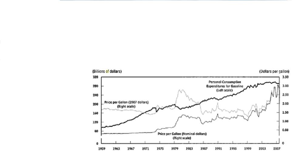
The graph above shows in January 2003 the average retail price for a gallon of gasoline here in the United States was $1.50; roughly equal to the real inflation adjusted price during much of the preceding half century. Since then, the price of gasoline here in the United States has risen sharply. It was last below $2 per gallon in February 2005, and for much of 2007, prices topped $3 per gallon.

The Congressional Budget Office study examines the scope and intensity of consumers’ responses to the upward trend in gasoline prices that began in 2003 as mentioned above. “Those responses have been large enough to interrupt a pattern of steady growth in total gasoline consumption dating back to 1990, the last time here in the United States where gasoline prices rose substantially” (Davis 2001). If current high prices and consumer’s responses to them persist, the effect on overall gasoline consumption will grow stronger as older; less fuel efficient vehicles are retired and as consumers consider other, less easily implemented adjustments to their patterns of consumptions.

The 55-mph speed limit policy is preferable. This is more preferable because motorists can reduce their fuel costs if they drive more slowly. The incentive to slow down will depend on how much gasoline prices have increase, how much fuel would be saved by slowing down, and how much motorists value their time while driving. The value of the potential fuel savings from slowing down is rather small compared with reasonable measures of many motorists’ value of time, so the likely effect of gasoline prices on highway speeds also should be rather small. For any given reduction in speed, however, the fuel savings are greater at faster speeds and for less-fuel-efficient vehicles.

References:

Davis, C. Stacy. (2001). Transportation Energy Data Book: Edition 21-2001, ORNL-6966.

Retrieved on May 23, 2013; from: http://cta.ornl.gov/cta/Publications/Reports/ORNL-6966.pdf

Dunn, William N., Public Policy Analysis, Pearson, 5th ed., 2012, p. 74, 246-253.

Minnesota Department of Transportation, 2003, "Per Mile Costs of Operating Automobiles and

Trucks,". Retrieved on May 22, 2013; from: http://trid.trb.org/view.aspx?id=678531

USDOT, April 9, 1997; Revised February 2003, "Departmental Guidance on the Evaluation of

Travel Time in Economic Analysis Memo;". Retrieved on May 22, 2013; from: http://www.

dot.gov/sites/dot.dev/files/docs/vot_guidance_092811c.pdf.

US DOT, 2003, "Revised Departmental Guide lines: Valuation of Travel Time in Economic

Analysis" memorandum. Retrieved on may 22, 2013; from: http://www.dot.gov/regulations

/economic-values-used-in-analysis