ARIMA-MODEL BY"IBM spss statistics 24"
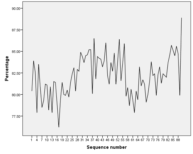
The first data set contains observations adapted from a series provided by a large U.S. corporation. There are 90 weekly observations showing the percentage of the time that parts for an industrial product are available when needed. The data can be found on Blackboard with “parts” as the pre-fix. Use the observation 1 to 85 for model building and assessing model goodness of fit for estimation purposes. Use the observation 86 to 90 for assessing model goodness of fit for forecasting purposes.
Fit a White Noise model to the original data and based on the results of Residuals ACF and Residuals PACF, select an initial model. Estimate the model parameters. Check the stationarity and invertibility conditions. Are the parameter estimates significant? Are the model assumptions satisfied? In efforts to approach White Noise series, improve your initial model by fitting another model based on the initial model results of Residuals ACF and Residuals PACF. Estimate the model parameters. Check the stationarity and invertibility conditions. Are the parameter estimates significant? Are the model assumptions satisfied?
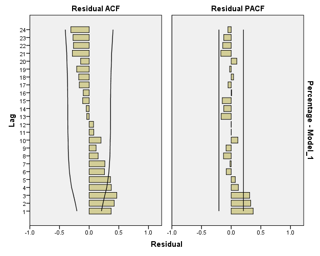
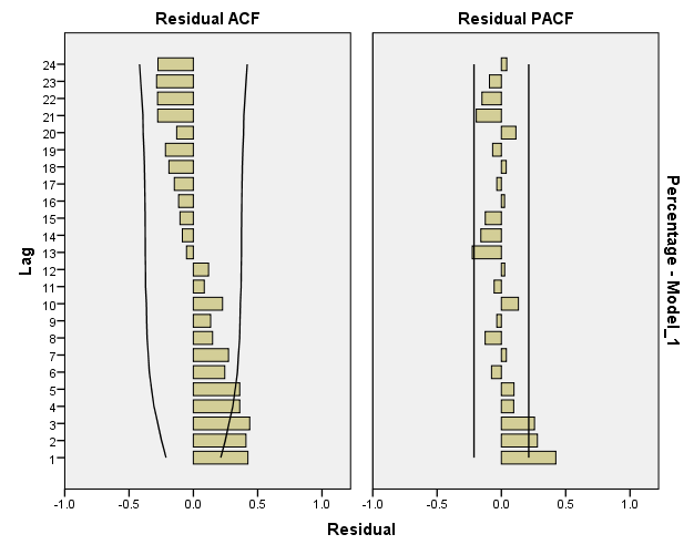
The sample ACF and PACF functions of original data seem to suggest that the data follow ARMA processes. Based on the principle of parsimony, we will start fitting an AR(1) process to the data. The summaries of the fit and diagnostics are listed below:
| Model Description | |||
| Model Type | |||
| Model ID | Percentage | Model_1 | ARIMA(1,0,0) |
| The Model Statistics | |||||||||||
| Model | Number of Predictors | Model Fit statistics | Ljung-Box Q(18) | Number of Outliers | |||||||
| Stationary R-squared | RMSE | MAPE | MAE | Statistics | DF | Sig. | |||||
| Percentage-Model_1 | 0 | .184 | 2.050 | 2.025 | 1.657 | 27.308 | 17 | .054 | 0 | ||
| ARIMA Model Parameters | ||||||||||||
| Estimate | SE | t | Sig. | |||||||||
| Percentage-Model_1 | Percentage | No Transformation | Constant | 81.982 | .387 | 211.660 | .000 | |||||
| AR | Lag 1 | .431 | .100 | 4.302 | .000 | |||||||
| Forecast | |||||||||||
| Model | 86 | 87 | 88 | 89 | 90 | ||||||
| Percentage-Model_1 | Forecast | 83.33 | 82.56 | 82.23 | 82.09 | 82.03 | |||||
| UCL | 87.40 | 87.00 | 86.73 | 86.60 | 86.54 | ||||||
| LCL | 79.25 | 78.12 | 77.73 | 77.58 | 77.51 | ||||||
Testing for significance of models parameters:
1/ State the null and alternate hypotheses.
H0: Ø1 = 0
H1: Ø1 ≠ 0
2/ State the decision rule, report the p-value.
level of significance (α) = 0.05. Since it is two-tailed test, reject H0 if P.V < 0.05/2 otherwise fail to reject H0
P-value = 0 (there is a small chance that the null hypothesis is true)
3/ What is your decision regarding the null hypothesis? Interpret the result.
Since P.V < 0.05/2 at 0.05 level of significance, we reject H0.
We conclude that the first parameter of AR(1) is contributing significantly into explaining the variation of the response variable (the percentage of the time that parts for an industrial product are available when needed)
Checking the stationarity conditions:
│ │<1
│<1
│0.431│<1 so the model is stationary.
Checking invertibility conditions:
AR processes are always invertible.
Checking model assumptions:
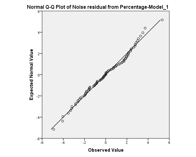
Normality of residuals:

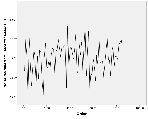
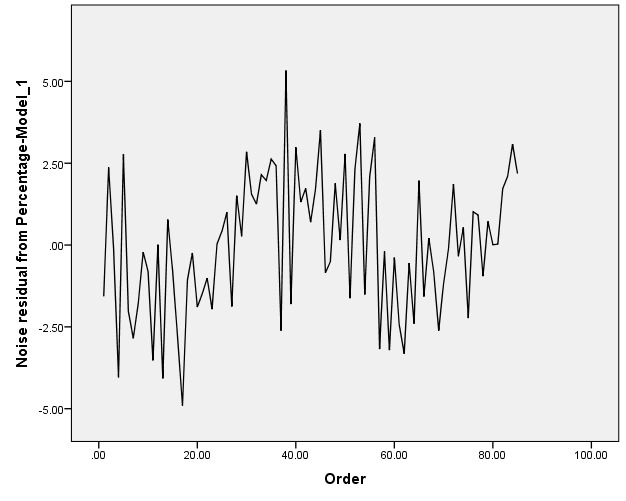
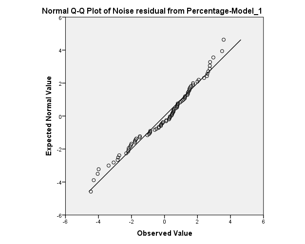
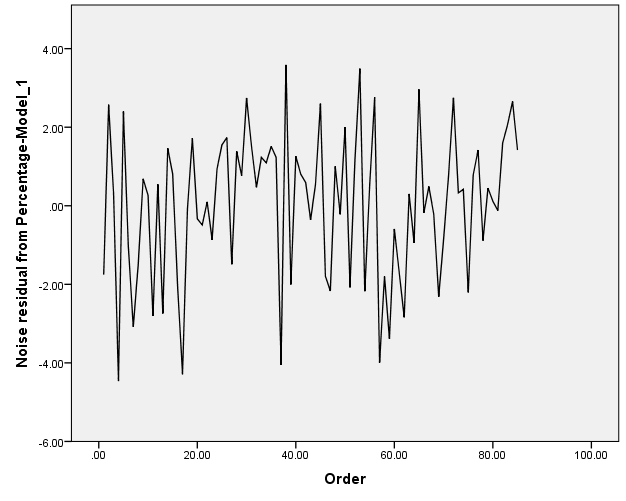
The normality assumption seems to be satisfied. However, there are two observation at the bottom and the top of the graph above may decrease the P.V of the goodness of fit test.
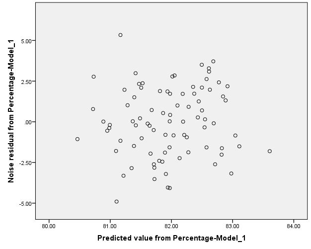
Constant variance of residuals:
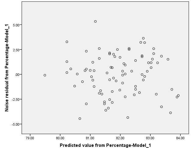
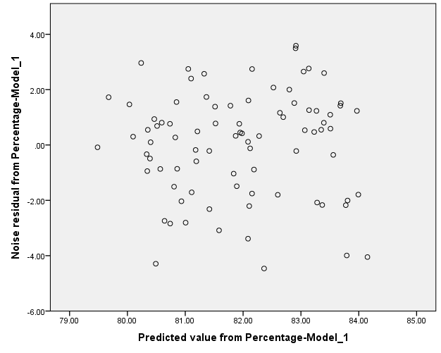
The constant variance of the residual terms seems to be satisfied since there is no megaphone shape is observed in the graph.
Independence of residuals:
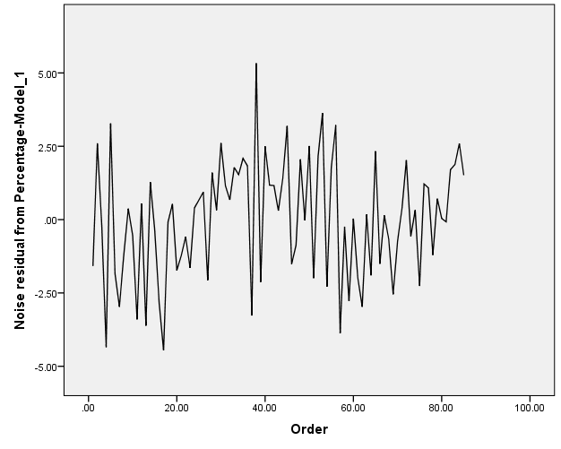
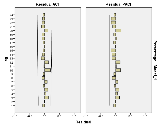
The graph above depicts a potentiality of having negative auto-correlation.
Reaching White-Noise Process:
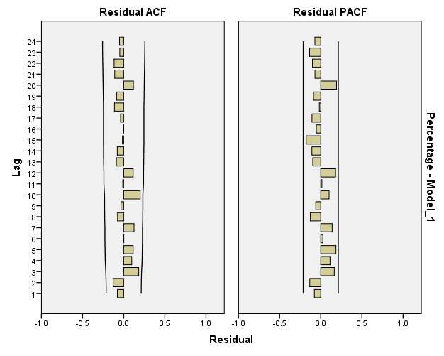
Looking at the Residual ACF and Residuals PACF, the model is close to White-Noise Series but it has not reached it yet; which suggest fitting more complex models.
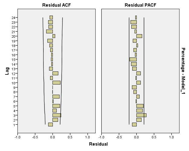
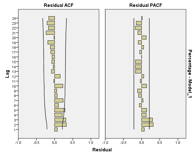
The sample ACF and PACF functions of residuals of AR(1) model seem to suggest that the data follow ARMA processes. we should try fitting an MA(1) process to the data. However, I chose to fit AR(2) process first then fit MA(1) and ARMA(1,1) later in the analysis. The summaries of the fit and diagnostics are listed below:
| Model Description | |||
| Model Type | |||
| Model ID | Percentage | Model_1 | ARIMA(2,0,0) |
| Model Statistics | |||||||||||
| Model | Number of Predictors | Model Fit statistics | Ljung-Box Q(18) | Number of Outliers | |||||||
| Stationary R-squared | RMSE | MAPE | MAE | Statistics | DF | Sig. | |||||
| Percentage-Model_1 | 0 | .253 | 1.973 | 1.910 | 1.561 | 17.523 | 16 | .353 | 0 | ||
| ARIMA Model Parameters | ||||||||||||
| Estimate | SE | t | Sig. | |||||||||
| Percentage-Model_1 | Percentage | No Transformation | Constant | 82.042 | .528 | 155.528 | .000 | |||||
| AR | Lag 1 | .305 | .105 | 2.897 | .005 | |||||||
| Lag 2 | .299 | .108 | 2.776 | .007 | ||||||||
| Forecast | |||||||||||
| Model | 86 | 87 | 88 | 89 | 90 | ||||||
| Percentage-Model_1 | Forecast | 84.07 | 83.57 | 83.12 | 82.83 | 82.60 | |||||
| UCL | 87.99 | 87.67 | 87.49 | 87.28 | 87.11 | ||||||
| LCL | 80.15 | 79.48 | 78.74 | 78.38 | 78.10 | ||||||
| | |||||||||||
Testing for significance of models parameters:
1/ State the null and alternate hypotheses.
H0: Øi = 0
H1: Øi ≠ 0 , i = 1,2
2/ State the decision rule, report the p-value.
level of significance (α) = 0.05. Since it is two-tailed test, reject H0 if P.V < 0.05/2 otherwise fail to reject H0
P-value (Ø1) = 0.005 (there is a small chance that the null hypothesis is true)
P-value (Ø2) = 0.007 (there is a small chance that the null hypothesis is true)
3/ What is your decision regarding the null hypothesis? Interpret the result.
Since P.V < 0.05/2 at 0.05 level of significance, we reject H0.
We conclude that the first and second parameters of AR(2) are contributing significantly into explaining the variation of the response variable (the percentage of the time that parts for an industrial product are available when needed)
Checking the stationarity conditions:
│ │<1
│<1
 < 1
< 1
 < 1
< 1
│0.299│<1
 < 1
< 1
 < 1
< 1
So the model is stationary.
Checking invertibility conditions:
AR processes are always invertible.
Checking model assumptions:
Normality of residuals:

The normality assumption seems to be satisfied.
Constant variance of residuals:
The constant variance of the residual term seems to be satisfied since there is no megaphone shape is observed in the graph.
Independence of residuals:
The graph above depicts a potentiality of having negative auto-correlation.
Reaching White-Noise Process:
Looking at the Residual ACF and Residuals PACF, the model has reached White-Noise Series
Select an alternative model (one that is different from your initial model) fit a White Noise model to the original data and based on the results of Residuals ACF and Residuals PACF. Estimate the model parameters. Check the stationarity and invertibility conditions. Are the parameter estimates significant? Are the model assumptions satisfied? In efforts to approach Whit Noise series, improve your alternative model by fitting another model based on the alternative model results of Residuals ACF and Residuals PACF. Estimate the model parameters. Check the stationarity and invertibility conditions. Are the parameter estimates significant? Are the model assumptions satisfied?
The sample ACF and PACF functions of original data seem to suggest that the data follow ARMA processes. Based on the principle of parsimony, we will start fitting an MA(1) process to the data. The summaries of the fit and diagnostics are listed below:
| Model Description | |||
| Model Type | |||
| Model ID | Percentage | Model_1 | ARIMA(0,0,1) |
| Model Statistics | |||||||||||
| Model | Number of Predictors | Model Fit statistics | Ljung-Box Q(18) | Number of Outliers | |||||||
| Stationary R-squared | RMSE | MAPE | MAE | Statistics | DF | Sig. | |||||
| Percentage-Model_1 | 0 | .122 | 2.126 | 2.118 | 1.734 | 49.784 | 17 | .000 | 0 | ||
| ARIMA Model Parameters | ||||||||||||
| Estimate | SE | t | Sig. | |||||||||
| Percentage-Model_1 | Percentage | No Transformation | Constant | 81.969 | .300 | 272.836 | .000 | |||||
| MA | Lag 1 | -.307 | .105 | -2.923 | .004 | |||||||
| Forecast | ||||||
| Model | 86 | 87 | 88 | 89 | 90 | |
| Percentage-Model_1 | Forecast | 82.64 | 81.97 | 81.97 | 81.97 | 81.97 |
| UCL | 86.87 | 86.39 | 86.39 | 86.39 | 86.39 | |
| LCL | 78.41 | 77.55 | 77.55 | 77.55 | 77.55 | |
Testing for significance of model parameters:
1/ State the null and alternate hypotheses.
H0: θ1 = 0
H1: θ1 ≠ 0
2/ State the decision rule, report the p-value.
level of significance (α) = 0.05. Since it is two-tailed test, reject H0 if P.V < 0.05/2 otherwise fail to reject H0
P-value = 0.004 (there is a small chance that the null hypothesis is true)
3/ What is your decision regarding the null hypothesis? Interpret the result.
Since P.V < 0.05/2 at 0.05 level of significance, we reject H0.
We conclude that the first parameter of MA(1) is contributing significantly into explaining the variation of the response variable (the percentage of the time that parts for an industrial product are available when needed)
Checking the stationarity conditions:
MA processes are always stationary.
Checking invertibility conditions:
│ │<1
│<1
│-.307│<1 so the model is invertible.
Checking model assumptions:
Normality of residuals:
The normality assumption seems to be satisfied. However, there are two observation at the bottom and the top of the graph above may decrease the P.V of the goodness of fit test.
Constant variance of residuals:
The constant variance of the residual term seems to be satisfied since there is no megaphone shape is observed in the graph.
Independence of residuals:
The graph above depicts a potentiality of having negative auto-correlation.
Reaching White-Noise Process:
Looking at the Residual ACF and Residuals PACF, the model is close to White-Noise Series but it has not reached it yet; which suggest fitting more complex models.
The sample ACF and PACF functions of residuals of MA(1) model seem to suggest that the data follow ARMA processes. we should try fitting an ARMA(1,1) process to the data. The summaries of the fit and diagnostics are listed below:
| Model Description | |||
| Model Type | |||
| Model ID | Percentage | Model_1 | ARIMA(1,0,1) |
| Model Statistics | |||||||||||
| Model | Number of Predictors | Model Fit statistics | Ljung-Box Q(18) | Number of Outliers | |||||||
| Stationary R-squared | RMSE | MAPE | MAE | Statistics | DF | Sig. | |||||
| Percentage-Model_1 | 0 | .300 | 1.910 | 1.869 | 1.527 | 13.924 | 16 | .604 | 0 | ||
| ARIMA Model Parameters | ||||||||||||||||
| Estimate | SE | t | Sig. | |||||||||||||
| Percentage-Model_1 | Percentage | No Transformation | Constant | 82.154 | .830 | 98.928 | .000 | |||||||||
| AR | Lag 1 | .920 | .070 | 13.188 | .000 | |||||||||||
| MA | Lag 1 | .654 | .130 | 5.015 | .000 | |||||||||||
| Forecast | ||||||
| Model | 86 | 87 | 88 | 89 | 90 | |
| Percentage-Model_1 | Forecast | 83.94 | 83.79 | 83.66 | 83.54 | 83.43 |
| UCL | 87.72 | 87.71 | 87.69 | 87.65 | 87.62 | |
| LCL | 80.15 | 79.88 | 79.64 | 79.43 | 79.24 | |
Testing for significance of model parameters:
1/ State the null and alternate hypotheses.
H0: Ø1 = 0
H1: Ø1 ≠ 0
H0: θ1 = 0
H1: θ1 ≠ 0
2/ State the decision rule, report the p-value.
level of significance (α) = 0.05. Since it is two-tailed test, reject H0 if P.V < 0.05/2 otherwise fail to reject H0
P-value (Ø1) = 0 (there is a small chance that the null hypothesis is true)
P-value (θ1) = 0 (there is a small chance that the null hypothesis is true)
3/ What is your decision regarding the null hypothesis? Interpret the result.
Since P.V < 0.05/2 at 0.05 level of significance, we reject H0.
We conclude that both parameters of ARMA(1,1) are contributing significantly into explaining the variation of the response variable (the percentage of the time that parts for an industrial product are available when needed)
Checking the stationarity conditions:
││<1
│0.920│<1 so the model is stationary.
Checking invertibility conditions:
││<1
│0.654│<1 so the model is invertible.
Checking model assumptions:
Normality of residuals:
The normality assumption seems to be moderately violated.
Constant variance of residuals:
The constant variance of the residual term seems to be satisfied since there is no megaphone shape is observed in the graph.
Independence of residuals:
The graph above depicts a potentiality of having negative auto-correlation.
Reaching White-Noise Process:
Looking at the Residual ACF and Residuals PACF, the model has reached White-Noise Series
c. Based on the results obtained from parts a and b, fill in the tables below to evaluate the potential models. Which model do you prefer for estimation purposes? Which model do you prefer for forecasting purposes?
| Checking Model Assumptions (Residuals) | ||||
| Model/ Measure | ARIMA (1,0,0) | AEIMA (2,0,0) | ARIMA (0,0,1) | ARIMA (1,0,1) |
| Normality | Satisfied | Satisfied | Satisfied | Moderately violated |
| Constant Variance | Satisfied | Satisfied | Satisfied | Satisfied |
| Independence | Moderately violated | Moderately violated | Moderately violated | Moderately violated |
| White noise | violated | Satisfied | violated | Satisfied |
| Model Stationarity | Satisfied | Satisfied | Satisfied | Satisfied |
| Model Invertibility | Satisfied | Satisfied | Satisfied | Satisfied |
The highlighted model does not suggest further refinement, while the other models suggest some refinements.
| Goodness of fit for (Estimation) | ||||
| Model/ Measure | ARIMA (1,0,0) | AEIMA (2,0,0) | ARIMA (0,0,1) | ARIMA (1,0,1) |
| RMSE | 2.050 | 1.973 | 2.126 | 1.910 |
| MAE | 1.657 | 1.561 | 1.734 | 1.527 |
| MAPE | 2.025 | 1.910 | 2.118 | 1.869 |
| Number of Parameters (Complexity) | ||||
| Number of Significant Parameters | ||||
The highlighted model is the best model for estimation purposes.
| Goodness of fit for (Forecasting) | ||||
| Model/ Measure | ARIMA (1,0,0) | AEIMA (2,0,0) | ARIMA (0,0,1) | ARIMA (1,0,1) |
| RMSE | 3.706869299 | 3.297838686 | 3.908943591 | 3.09327658 |
| MAE | 3.148 | 2.618 | 3.444 | 2.504 |
| MAPE | 0.036641804 | 0.030578392 | 0.040101984 | 0.029427493 |
The highlighted model is the best model for forecasting purposes.
Use the entire data set and based on your best model for forecasting, forecast the observations: 91, 92, 93, 94, and 95. Provide both a point estimate and a confidence interval for each forecasted observation.
| Forecast | ||||||
| Model | 91 | 92 | 93 | 94 | 95 | |
| Percentage-Model_1 | Forecast | 84.44 | 84.29 | 84.16 | 84.03 | 83.92 |
| UCL | 88.45 | 88.43 | 88.39 | 88.36 | 88.31 | |
| LCL | 80.43 | 80.16 | 79.92 | 79.71 | 79.52 | |
| | ||||||
1. The data set contains the monthly total (in thousands) of persons unemployed in Canada from January 1956 to December 1975. There are a total of 240 observations. The data can be found on Blackboard with “Unemployment-Canada” as the title. Use the observation 1 to 230 for model building and assessing model goodness of fit for estimation purposes. Use the observation 231 to 240 for assessing model goodness of fit for forecasting purposes.
a. Fit a White Noise model to the original data and based on the results of Residuals ACF and Residuals PACF, select an initial model for both seasonal components and non-seasonal components. Estimate the model parameters. Check the stationarity and invertibility conditions. Are the parameter estimates significant? Are the model assumptions satisfied? In efforts to approach White Noise series, improve your initial model by fitting another model both seasonal components and non-seasonal components based on the initial model results of Residuals ACF and Residuals PACF. Estimate the model parameters. Check the stationarity and invertibility conditions. Are the parameter estimates significant? Are the model assumptions satisfied?
Instead of doing part (a), you could run a several models aiming to reach White Noise series. Examine each model Residuals ACF and Residuals PACF.
| Model Description | ||||
| Model Type | ||||
| Model ID | Unemp | Model_1 | ARIMA(0,0,0)(0,0,0) | |
| Model Statistics | |||||||||||
| Model | Number of Predictors | Model Fit statistics | Ljung-Box Q(18) | Number of Outliers | |||||||
| Stationary R-squared | RMSE | MAPE | MAE | Statistics | DF | Sig. | |||||
| Unemp-Model_1 | 0 | -2.168E-19 | 144.154 | 37.342 | 119.948 | 920.567 | 18 | .000 | 0 | ||
| ARIMA Model Parameters | |||||||||||
| Estimate | SE | t | Sig. | ||||||||
| Unemp-Model_1 | Unemp | No Transformation | Constant | 401.561 | 9.505 | 42.246 | .000 | ||||
| Model Description | |||
| Model Type | |||
| Model ID | Unemployment | Model_1 | ARIMA(0,0,0)(1,0,0) |
| Model Description | |||
| Model Type | |||
| Model ID | Unemployment | Model_1 | ARIMA(1,0,0)(1,0,0) |
| Model Description | |||
| Model Type | |||
| Model ID | Unemployment | Model_1 | ARIMA(1,0,1)(1,0,0) |

| Model Description | |||
| Model Type | |||
| Model ID | Unemployment | Model_1 | ARIMA(1,0,1)(1,0,1) |
| Model Description | |||
| Model Type | |||
| Model ID | Unemployment | Model_1 | ARIMA(2,0,1)(1,0,1) |
| Model Description | |||
| Model Type | |||
| Model ID | Unemployment | Model_1 | ARIMA(2,0,2)(1,0,1) |
| Model Description | |||
| Model Type | |||
| Model ID | Unemployment | Model_1 | ARIMA(2,0,2)(2,0,1) |
| Model Description | |||
| Model Type | |||
| Model ID | Unemployment | Model_1 | ARIMA(2,0,2)(2,0,2) |
| Model Description | |||
| Model Type | |||
| Model ID | Unemployment | Model_1 | ARIMA(2,1,2)(2,0,2) |
| Model Description | |||
| Model Type | |||
| Model ID | Unemployment | Model_1 | ARIMA(2,0,2)(2,1,2) |
| Model Description | |||
| Model Type | |||
| Model ID | Unemployment | Model_1 | ARIMA(2,1,2)(2,1,2) |
Do this part if you chose to do part (a) only. Select an alternative model (one that is different from your initial model) fit a White Noise model to the original data and based on the results of Residuals ACF and Residuals PACF. Estimate the model parameters. Check the stationarity and invertibility conditions. Are the parameter estimates significant? Are the model assumptions satisfied? In efforts to approach Whit Noise series, improve your alternative model by fitting another model based on the alternative model results of Residuals ACF and Residuals PACF. Estimate the model parameters. Check the stationarity and invertibility conditions. Are the parameter estimates significant? Are the model assumptions satisfied?
Do this part if you chose to do part (b) only. Select one of the best models you have from part (b) as initial model. For further diagnosis, estimate the model parameters. Check the stationarity and invertibility conditions. Are the parameter estimates significant? Are the model assumptions satisfied? Then select another good model you have from part (b) as alternative model. For further diagnosis, estimate the model parameters. Check the stationarity and invertibility conditions. Are the parameter estimates significant? Are the model assumptions satisfied?
| Model Description | ||||
| Model Type | ||||
| Model ID | Unemployment | Model_1 | ARIMA(2,0,1)(1,0,1) | |
| Model Statistics | |||||||||||
| Model | Number of Predictors | Model Fit statistics | Ljung-Box Q(18) | Number of Outliers | |||||||
| Stationary R-squared | RMSE | MAPE | MAE | Statistics | DF | Sig. | |||||
| Unemployment-Model_1 | 0 | .965 | 27.290 | 5.950 | 20.340 | 29.929 | 13 | .005 | 0 | ||
| ARIMA Model Parameters | ||||||||||||
| Estimate | SE | t | Sig. | |||||||||
| Unemployment-Model_1 | Unemployment | No Transformation | Constant | 437.249 | 305.087 | 1.433 | .153 | |||||
| AR | Lag 1 | 1.609 | .225 | 7.140 | .000 | |||||||
| Lag 2 | -.635 | .217 | -2.925 | .004 | ||||||||
| MA | Lag 1 | .461 | .259 | 1.778 | .077 | |||||||
| AR, Seasonal | Lag 1 | .977 | .013 | 77.173 | .000 | |||||||
| MA, Seasonal | Lag 1 | .516 | .077 | 6.689 | .000 | |||||||
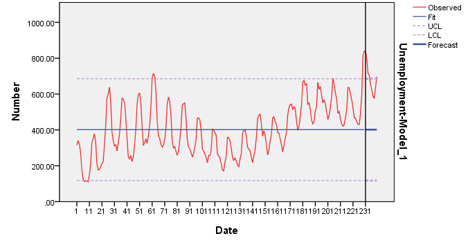
| Forecast | |||||||||||
| Model | Mar 1919 | Apr 1919 | May 1919 | Jun 1919 | Jul 1919 | Aug 1919 | Sep 1919 | Oct 1919 | Nov 1919 | Dec 1919 | |
| Unemployment-Model_1 | Forecast | 820.26 | 790.10 | 730.27 | 701.01 | 671.28 | 631.90 | 599.36 | 593.84 | 632.02 | 691.27 |
| UCL | 867.92 | 862.66 | 823.04 | 810.57 | 794.84 | 767.11 | 744.26 | 746.79 | 791.67 | 856.50 | |
| LCL | 772.61 | 717.53 | 637.49 | 591.44 | 547.72 | 496.69 | 454.46 | 440.88 | 472.36 | 526.04 | |
| For each model, forecasts start after the last non-missing in the range of the requested estimation period, and end at the last period for which non-missing values of all the predictors are available or at the end date of the requested forecast period, whichever is earlier. | |||||||||||
Testing for significance of model parameters (Seasonal Components) ARIMA (1,0,1)12:
1/ State the null and alternate hypotheses.
H0: Ø12 = 0
H1: Ø12 ≠ 0
H0: θ12 = 0
H1: θ12 ≠ 0
2/ State the decision rule, report the p-value.
level of significance (α) = 0.05. Since it is two-tailed test, reject H0 if P.V < 0.05/2 otherwise fail to reject H0
P-value (Ø12) = 0 (there is a small chance that the null hypothesis is true)
P-value (θ12) = 0 (there is a small chance that the null hypothesis is true)
3/ What is your decision regarding the null hypothesis? Interpret the result.
Since P.V < 0.05/2 at 0.05 level of significance, we reject H0.
We conclude that both parameters of ARIMA(1,0,1)12 are contributing significantly into explaining the seasonal variation of the response variable (the monthly total (in thousands) of persons unemployed in Canada from January 1956 to December 1975)
Checking the stationarity conditions:
│ │<1
│<1
│0.977│<1 so the seasonal model is stationary.
Checking invertibility conditions:
││<1
│0.516│<1 so the seasonal model is invertible.
Testing for significance of models parameters (Non-Seasonal Components) ARIMA (2,0,1):
1/ State the null and alternate hypotheses.
H0: Øi = 0
H1: Øi ≠ 0 , i = 1,2
H0: θ1 = 0
H1: θ1 ≠ 0
2/ State the decision rule, report the p-value.
level of significance (α) = 0.05. Since it is two-tailed test, reject H0 if P.V < 0.05/2 otherwise fail to reject H0
P-value (Ø1) = 0.000 (there is a small chance that the null hypothesis is true)
P-value (Ø2) = 0.004 (there is a small chance that the null hypothesis is true)
P-value (θ1) = 0.077 (there is a chance that the null hypothesis is true)
3/ What is your decision regarding the null hypothesis? Interpret the result.
Since P.V < 0.05/2 at 0.05 level of significance, we reject H0.
We conclude that the first and second parameters of AR(2) are contributing significantly into explaining the variation of the response variable (the monthly total (in thousands) of persons unemployed in Canada from January 1956 to December 1975). However, the first parameter of MA(1) is not contributing significantly into explaining the variation of the response variable.
Checking the stationarity conditions:
││<1
< 1
< 1
│-0.635│<1
 < 1
< 1
 < 1
< 1
So the non-seasonal model is stationary.
Checking invertibility conditions:
││<1
│0.461│<1 so the non-seasonal model is invertible.
Checking model assumptions:
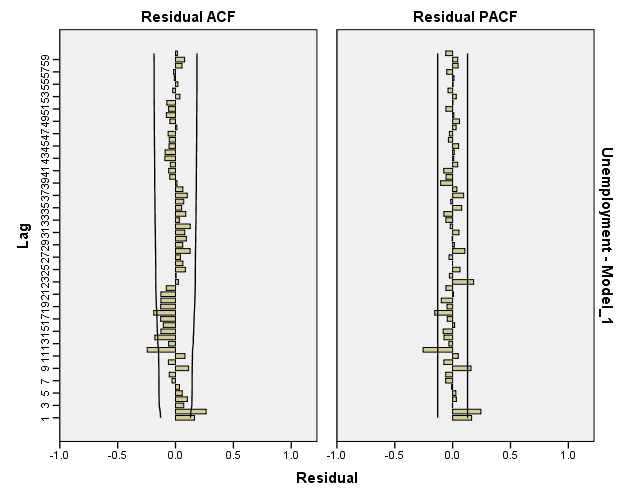
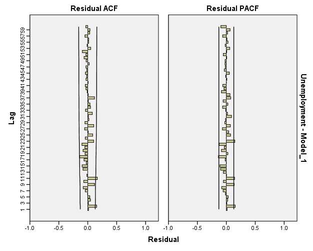
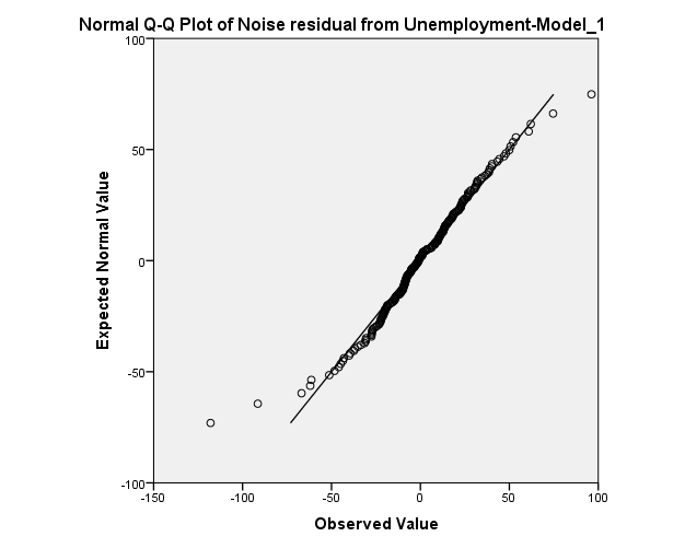
Normality of residuals:
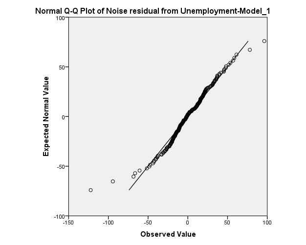
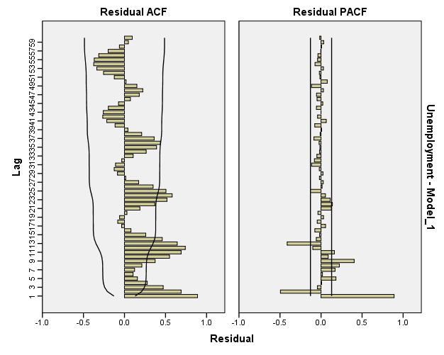
The normality assumption seems to be satisfied. However, there are two observation at the top and the bottom of the graph above may decrease the P.V of the goodness of fit test.
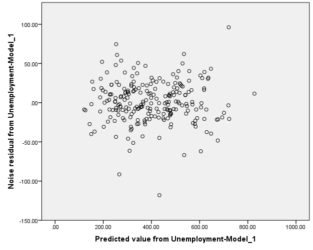
Constant Variance:
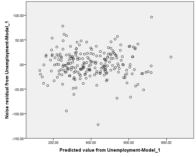
The constant variance of the residual term seems to be satisfied since there is no megaphone shape is observed in the graph.
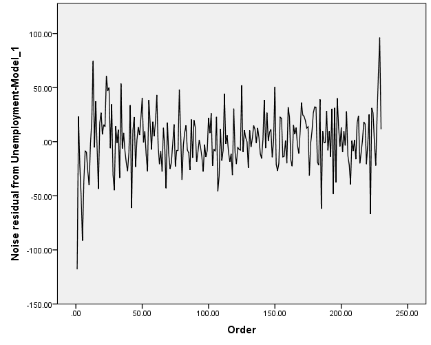
Independence of residuals:
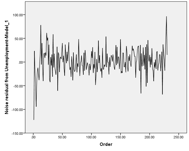
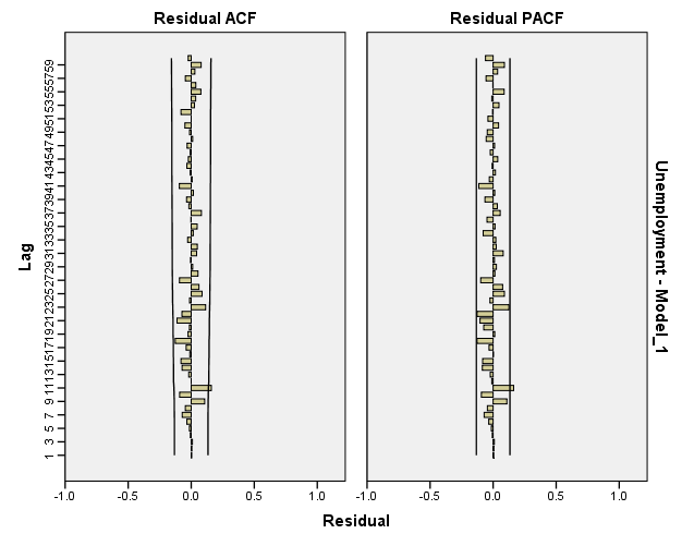
The graph above depicts a potentiality of having negative auto-correlation.
Reaching White-Noise Process:
Looking at the Residual ACF and Residuals PACF, the model is so close to White-Noise Series
| Model Description | ||||
| Model Type | ||||
| Model ID | Unemployment | Model_1 | ARIMA(2,0,2)(1,0,1) | |
| Model Statistics | |||||||||||
| Model | Number of Predictors | Model Fit statistics | Ljung-Box Q(18) | Number of Outliers | |||||||
| Stationary R-squared | RMSE | MAPE | MAE | Statistics | DF | Sig. | |||||
| Unemployment-Model_1 | 0 | .966 | 26.975 | 5.841 | 20.066 | 23.993 | 12 | .020 | 0 | ||
| ARIMA Model Parameters | ||||||||||||
| Estimate | SE | t | Sig. | |||||||||
| Unemployment-Model_1 | Unemployment | No Transformation | Constant | 433.010 | 290.024 | 1.493 | .137 | |||||
| AR | Lag 1 | 1.227 | .284 | 4.314 | .000 | |||||||
| Lag 2 | -.278 | .273 | -1.017 | .310 | ||||||||
| MA | Lag 1 | .118 | .280 | .422 | .674 | |||||||
| Lag 2 | -.208 | .085 | -2.463 | .015 | ||||||||
| AR, Seasonal | Lag 1 | .972 | .015 | 65.785 | .000 | |||||||
| MA, Seasonal | Lag 1 | .490 | .078 | 6.307 | .000 | |||||||
| Forecast | |||||||||||||||||||||
| Model | Mar 1919 | Apr 1919 | May 1919 | Jun 1919 | Jul 1919 | Aug 1919 | Sep 1919 | Oct 1919 | Nov 1919 | Dec 1919 | |||||||||||
| Unemployment-Model_1 | Forecast | 827.88 | 793.11 | 727.08 | 691.14 | 659.01 | 619.32 | 587.40 | 581.99 | 621.33 | 682.89 | ||||||||||
| UCL | 875.29 | 863.90 | 820.66 | 802.56 | 784.25 | 755.45 | 732.29 | 733.99 | 779.20 | 845.65 | |||||||||||
| LCL | 780.48 | 722.32 | 633.50 | 579.72 | 533.77 | 483.18 | 442.52 | 429.98 | 463.45 | 520.14 | |||||||||||
| For each model, forecasts start after the last non-missing in the range of the requested estimation period, and end at the last period for which non-missing values of all the predictors are available or at the end date of the requested forecast period, whichever is earlier. | |||||||||||||||||||||
Testing for significance of model parameters (Seasonal Components) ARIMA (1,0,1)12:
1/ State the null and alternate hypotheses.
H0: Ø12 = 0
H1: Ø12 ≠ 0
H0: θ12 = 0
H1: θ12 ≠ 0
2/ State the decision rule, report the p-value.
level of significance (α) = 0.05. Since it is two-tailed test, reject H0 if P.V < 0.05/2 otherwise fail to reject H0
P-value (Ø12) = 0 (there is a small chance that the null hypothesis is true)
P-value (θ12) = 0 (there is a small chance that the null hypothesis is true)
3/ What is your decision regarding the null hypothesis? Interpret the result.
Since P.V < 0.05/2 at 0.05 level of significance, we reject H0.
We conclude that both parameters of ARIMA(1,0,1)12 are contributing significantly into explaining the seasonal variation of the response variable (the monthly total (in thousands) of persons unemployed in Canada from January 1956 to December 1975)
Checking the stationarity conditions:
││<1
│0.972│<1 so the seasonal model is stationary.
Checking invertibility conditions:
││<1
│0.490│<1 so the seasonal model is invertible.
Testing for significance of models parameters (Non-Seasonal Components) ARIMA (2,0,1):
1/ State the null and alternate hypotheses.
H0: Øi = 0
H1: Øi ≠ 0 , i = 1,2
H0: θj = 0
H1: θj ≠ 0 , j = 1,2
2/ State the decision rule, report the p-value.
level of significance (α) = 0.05. Since it is two-tailed test, reject H0 if P.V < 0.05/2 otherwise fail to reject H0
P-value (Ø1) = 0.000 (there is a small chance that the null hypothesis is true)
P-value (Ø2) = 0.310 (there is a big chance that the null hypothesis is true)
P-value (θ1) = 0.674 (there is a big chance that the null hypothesis is true)
P-value (θ2) = 0.015 (there is a small chance that the null hypothesis is true)
3/ What is your decision regarding the null hypothesis? Interpret the result.
Since P.V < 0.05/2 at 0.05 level of significance, we reject H0.
We conclude that the first parameter of AR(2) is contributing significantly into explaining the variation of the response variable (the monthly total (in thousands) of persons unemployed in Canada from January 1956 to December 1975) while the second parameter is not significant. However, the first parameter of MA(2) is not contributing significantly into explaining the variation of the response variable, while the second parameter is significant.
Checking the stationarity conditions:
││<1
< 1
< 1
│-0.278│<1
 < 1
< 1
 < 1
< 1
So the non-seasonal model is stationary.
Checking invertibility conditions:
│ │<1
│<1
 < 1
< 1
 < 1
< 1
│-0.208│<1
 < 1
< 1
 < 1
< 1
So the non-seasonal model is invertible.
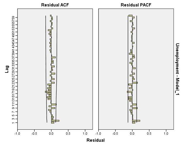
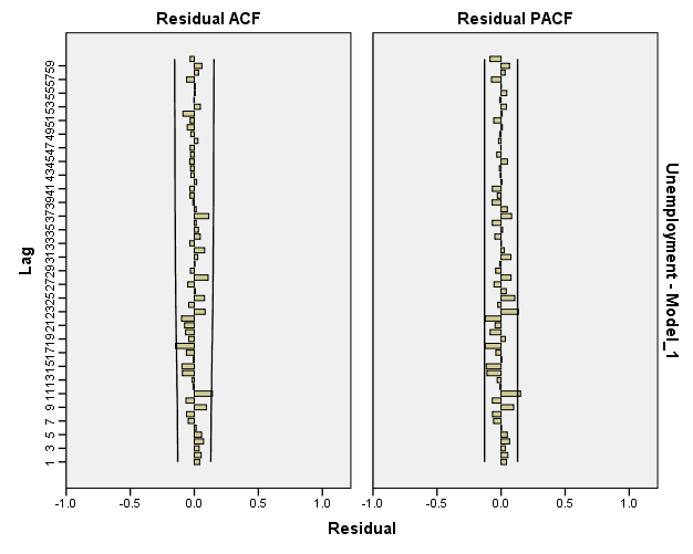
Checking model assumptions:
Normality of residuals:
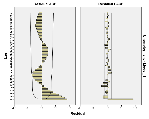
The normality assumption seems to be satisfied. However, there are two observation at the top and the bottom of the graph above may decrease the P.V of the goodness of fit test.
Constant Variance:
The constant variance of the residual term seems to be satisfied since there is no megaphone shape is observed in the graph.
Independence of residuals:
The graph above depicts a potentiality of having negative auto-correlation.
Reaching White-Noise Process:
Looking at the Residual ACF and Residuals PACF, the model is so close to White-Noise Series
Based on the results obtained from parts (a and c) or (b and d), fill in the tables below to evaluate the potential models. Which model do you prefer for estimation purposes? Which model do you prefer for forecasting purposes?
| Model/ Measure | ARIMA (2,0,1)(1,0,1)12 | AEIMA (2,0,2)(1,0,1)12 |
| Normality | Moderately violated | Moderately violated |
| Constant Variance | Satisfied | Satisfied |
| Independence | Moderately violated | Moderately violated |
| White noise | Moderately violated | Moderately violated |
| Model Stationarity | Satisfied | Satisfied |
| Model Invertibility | Satisfied | Satisfied |
Both models perform equally well and suggest further refinements.
| Model/ Measure | ARIMA (2,0,1)(1,0,1)12 | AEIMA (2,0,2)(1,0,1)12 |
| RMSE | 27.290 | 26.975 |
| MAE | 20.340 | 20.066 |
| MAPE | 5.950 | 5.841 |
| Number of Parameters (Complexity) | ||
| Number of Significant Parameters |
The highlighted model is the best model for estimation purposes since the two models are really close to each other in terms of accuracy; however the first model is less complex. .
| Model/ Measure | ARIMA (2,0,1)(1,0,1)12 | AEIMA (2,0,2)(1,0,1)12 |
| RMSE | 13.01525067 | 10.59290376 |
| MAE | 11.599 | 8.981 |
| MAPE | 0.017343794 | 0.013070704 |
The highlighted model is the best model for forecasting purposes.
Use the entire data set and based on your best model for forecasting, forecast the observations: 241 to 252. Provide both a point estimate and a confidence interval for each forecasted observation.
| Forecast | |||||||||||||
| Model | Jan 1920 | Feb 1920 | Mar 1920 | Apr 1920 | May 1920 | Jun 1920 | Jul 1920 | Aug 1920 | Sep 1920 | Oct 1920 | Nov 1920 | Dec 1920 | |
| Unemployment-Model_1 | Forecast | 852.54 | 847.45 | 825.01 | 780.70 | 708.01 | 686.01 | 646.41 | 612.44 | 579.33 | 572.89 | 623.17 | 681.14 |
| UCL | 899.24 | 917.02 | 917.17 | 890.31 | 831.13 | 819.83 | 788.89 | 762.04 | 734.87 | 733.39 | 787.87 | 849.41 | |
| LCL | 805.84 | 777.89 | 732.86 | 671.08 | 584.89 | 552.19 | 503.93 | 462.83 | 423.80 | 412.38 | 458.46 | 512.87 | |


