1. What is the difference between accounting profit and economic profit? How could a firm earn positive accounting profit but negative economic profit?2. Why is the marginal revenue of a perfectly c
Solutions to Chapter 9 Questions
Review Questions
1. What is the difference between accounting profit and economic profit? How could a firm earn positive accounting profit but negative economic profit?
The difference between accounting profit and economic profit is in how total cost is measured. With accounting profit, total cost is measured as total accounting cost while with economic profit, total cost is measured as total economic cost. Accounting cost measures the historical expenses the firm incurred to produce and sell its product while economic cost measured the opportunity cost of the resources that the firm uses to produce and sell its product.
If a firm chose to produce and sell a product it could earn a positive accounting profit but negative economic profit. This would occur if the economic cost of the resources used was greater than the accounting cost of the resources used. For example, the firm might purchase resources for $1 million and use these to produce a product when instead the firm could have resold the resources for $2 million. In this case the economic cost exceeds the accounting cost and economic profit would be less than accounting profit.
2. Why is the marginal revenue of a perfectly competitive firm equal to the market price?
The law of one price ensures that all transactions will take place at a single market price. A perfectly competitive firm cannot affect the market price by increasing or decreasing production. Therefore, for each unit produced and sold, the firm will receive the market price as revenue. Revenue will increase with each unit sold by the market price, implying the market price is equal to marginal revenue.
3. Would a perfectly competitive firm produce if price were less than the minimum level of average variable cost? Would it produce if price were less than the minimum level of short-run average cost?
A perfectly competitive firm would not produce if the market price is below the minimum of its average variable cost. If the firm shuts down, the “bad news” is that it loses revenue. The “good news” is that the firm avoids non-sunk costs (including variable costs). If the market price is below the minimum of the firm’s average variable cost, the good news from shutting down outweighs the bad news.
If the market price is below the minimum of the firm’s short-run average cost, the decision as to whether the firm should shut down depends on how much of the fixed costs are non-sunk (avoidable). Suppose first that all of the fixed costs are non-sunk. If the firm shuts down, the “bad news” is that it loses revenue. The “good news” is that the firm avoids variable costs, as well as all of the fixed costs. If the market price is below the minimum of the firm’s short-run average cost, the good news from shutting down outweighs the bad news.
Now suppose that some of the fixed costs are sunk. Then for at least some levels of market price below the minimum of short-run average cost, the revenue lost may be greater than the costs that can be avoided if the firm shuts down. For such a market price, the firm would be better off continuing to operate in the short-run, because its losses from operating would be less than the losses it would sustain if it were to shut down.
4. What is the shutdown price when all fixed costs are sunk? What is the shutdown price when all fixed costs are nonsunk?
When all fixed costs are sunk, the shut-down price is the minimum level of average variable cost. When all fixed costs are non-sunk, the shut-down price is the minimum level of short-run average cost.
10. Explain the difference between the following concepts: producer surplus, economic profit, and economic rent.
Producer surplus and economic profit may be equal in the short run. In particular, in the short run,
Producer Surplus = Economic Profit + Sunk Fixed Costs.
Thus, in the short run producer surplus and economic profits differ by the level of sunk fixed costs. However, in the long run, since no fixed costs are sunk, producer surplus and economic profit will be equal. In general, producer surplus measures the difference between total revenue and total non-sunk costs while economic profit measures the difference between total revenue and all total costs.
These two measures differ from economic rent. Economic rent is the economic surplus that is attributable to an extraordinarily productive input whose supply is limited. Essentially, economic rent measures the potential increase in economic profit attributable to the scarce input above and beyond the economic profit the firm would enjoy if the firm paid suppliers of the input an amount equal to their reservation value. However, it is possible that the input, because of its scarcity, can extract the economic rent from the firm so that the firm still earns zero economic profit.
Problem Questions
9.5. A competitive, profit-maximizing firm operates at a point where its short-run average cost curve is upward sloping. What does this imply about the firm’s economic profits? Briefly explain.
If the firm operates at a point where its SRAC curve is rising, it must mean that the SRMC curve lies above the SRAC curve. And since the firm will choose an output such that price=SRMC, it means that price is greater than SRAC. Therefore the firm is earning positive economic profit.
9.8 Dave’s Fresh Catfish is a northern Mississippi farm that operates in the perfectly competitive catfish farming industry. Dave’s short-run total cost curve is  2, where
  is the number of catfish harvest per month. The corresponding short-run marginal cost curve is
  . All of the fixed costs are sunk.
What is the equation for the average variable cost (
 )?
)?What is the minimum level of average variable costs?
What is Dave’s short-run supply curve?
 so
so 
The minimum level of
occurs at the where  , or
, or  , or
, or  . The minimum level of AVC is thus 2.
Since all fixed costs are sunk, the firm will not produce if the price is below the minimum level of
., or 2. For prices above 2, the quantity supplied is found by equation price to marginal cost, or  , which implies
  . Thus, the firm’s short-run supply curve is
 .
.
9.9. Ron’s Window Washing Service is a small business that operates in the perfectly competitive residential window washing industry in Evanston, Illinois. The short-run total cost of production is STC(Q) = 40+ 10Q + 0.1Q2, where Q is the number of windows washed per day. The corresponding short-run marginal cost function is SMC(Q) = 10 + 0.2Q. The prevailing market price is $20 per window.
a) How many windows should Ron wash to maximize profit?
b) What is Ron’s maximum daily profit?
c) Graph SMC, SAC, and the profit-maximizing quantity. On this graph, indicate the maximum daily profit.
d) What is Ron’s short-run supply curve, assuming that all of the $40 per day fixed costs are sunk?
e) What is Ron’s short-run supply curve, assuming that if he produces zero output, he can rent or sell his fixed assets and therefore avoid all his fixed costs?
a) In order to maximize profit Ron should operate at the point where  .
.

b) Ron’s profit is given by  .
.

c) The firm’s profit is equal to the shaded area in the graph below. It is a rectangle whose height is the market price and the average cost of the 50th unit, and whose width is the 50 units being produced.


d) If all fixed costs are sunk, then ANSC = AVC = (10Q + 0.1Q2)/Q = 10 + 0.1Q. So the first step is to find the minimum of ANSC by setting ANSC = SMC, or 10 + 0.1Q = 10 + 0.2Q which occurs when Q = 0. The minimum level of ANSC is thus 10. For prices below 10 the firm will not produce and for prices above 10, its supply curve is found by setting P = SMC:

The firm’s short-run supply curve is thus

e) If all fixed costs are non-sunk, as in this case, then ANSC = ATC = (40/Q) + 10 + 0.1Q. The minimum point of ANSC occurs where ANSC = SMC:

The minimum level of ANSC is thus 14. For prices below 14 the firm will not produce and for prices above 14, its supply curve is found by setting P = SMC as before.

9.10. The bolt-making industry currently consists of 20 producers, all of whom operate with the identical short-run total cost curve STC(Q) = 16 + Q2, where Q is the annual output of a firm. The corresponding short-run marginal cost curve is SMC(Q) = 2Q. The market demand curve for bolts is D(P) = 110 − P, where P is the market price.
a) Assuming that all of each firm’s $16 fixed cost is sunk, what is a firm’s short-run supply curve?
b) What is the short-run market supply curve?
c) Determine the short-run equilibrium price and quantity in this industry.
a) First, find the minimum of  by setting
  .
.

The minimum level of is thus 0. When the price is 0 the firm will produce 0, and for prices above 0 find supply by setting  .
.

Thus,

b) Market supply is found by horizontally summing the supply curves of the individual firms. Since there are 20 identical producers in this market, market supply is given by

c) Equilibrium price and quantity occur at the point where  .
.

Substituting  back into
  implies equilibrium quantity is
  . So at the equilibrium, and .
9.12. The oil drilling industry consists of 60 producers, all of whom have an identical short-run total cost curve, STC(Q) = 64 + 2Q2, where Q is the monthly output of a firm and $64 is the monthly fixed cost. The corresponding short-run marginal cost curve is SMC(Q) = 4Q. Assume that $32 of the firm’s monthly $64 fixed cost can be avoided if the firm produces zero output in a month. The market demand curve for oil drilling services is D(P) = 400 − 5P, where D(P) is monthly demand at price P. Find the market supply curve in this market, and determine the short-run equilibrium price.
The firm’s ANSC curve is given by 32/Q + 2Q. To find the shut-down price, we find the minimum level of ANSC. This occurs at the quantity at which ANSC equals MC, or
32/Q + 2Q = 4Q. Solving for Q yields Q = 4, and substituting this into the expression for ANSC tells us that the minimum level of ANSC is equal to 32/4 + 2(4) = $8. At prices below $8, a firm’s supply is 0. At prices above $8, a firm produces a quantity at which
P = SMC: P = 4Q, or Q = P/4. Thus, the short-run supply curve for a firm is:

Since there are 60 identical producers, each with this supply curve, the short-run market supply curve S(P) is 60 times s(P), or:

To find the equilibrium price, we equate market supply to market demand and solve for P: 15P = 400 – 5P, or P = 20.
9.14. A perfectly competitive industry consists of two types of firms: 100 firms of type A and 30 firms of type B. Each type A firm has a short-run supply curve sA(P) = 2P. Each type B firm has a short-run supply curve sB(P) = 10P. The market demand curve is D(P) = 5000 − 500P. What is the short-run equilibrium price in this market? At this price, how much does each type A firm produce, and how much does each type B firm produce?
Total industry supply is the sum of the supply curves of the individual firms. Since we have 100 type A firms, total supply from type A firms is 100sA(P) = 200P, and since we have 30 type B firms, total supply from type B firms is 30sB(P) = 300P. The short-run industry supply curve is thus S(P) = 200P + 300P = 500P. The short-run market equilibrium occurs at the price at which quantity supplied equals quantity demanded, or 5000 – 500P = 500P, or P = 5. At this price, a type A firm supplies 10 units, while a type B firm supplies 50 units.
9.18. A firm in a competitive industry produces its output in two plants. Its total cost of producing Q1 units from the first plant is TC1 = (Q1)2, and the marginal cost at this plant is MC1 = 2Q1. The firm’s total cost of producing Q2 units from the second plant is TC2 = 2(Q2)2; the marginal cost at this plant is MC2 = 4Q2. The price in the market is P. What fraction of the firm’s total supply will be produced at plant 2?
Given a market price P, the firm will produce from each plant so that MC = P.
The profit maximizing quantity supplied at plant 1 will be 2Q1 = P, or Q1 = P/2.
The profit maximizing quantity supplied at plant 2 will be 4Q2 = P, or Q2 = P/4.
The quantity supplied by the whole firm will QFirm = Q1 + Q2. Thus QFirm = 3P/4.
So 1/3 of the firm’s total production will come from plant 2.
9.19. A competitive industry consists of 6 type A firms and 4 type B firms. Each firm of type A operates with the supply curve:
![]()
Each firm of type B operates with the supply curve:
![]()
a) Suppose the market demand is ![]()
At the market equilibrium, which firms are producing, and what is the equilibrium price?
b) Suppose the market demand is ![]()
At the market equilibrium, which firms are producing, and what is the equilibrium price?
a) When P <10, only Type B firms will operate, and the market supply will be 4(2P) = 8P.
When P >10, both types of firms will operate, and the market supply will be
4(2P) + 6(-10 + P) = -60 + 14P.
To summarize, the market supply will be 
Let’s first assume the equilibrium price exceeds 10, so that all firms are producing. If this is true, setting market supply equal to market demand: -60 + 14P = 108 – 10P, so that P = 7; however, the market supply we have used is valid for P>10, but not valid for P = 7.
So the equilibrium price must be less than 10, with only Type B firms producing (and Type A firms not producing).
Setting market supply equal to market demand: 8P = 108 – 10P, so that P = 6.
We have found that in equilibrium, only Type B firms produce, and the equilibrium price is 6.
b) Let’s first assume the equilibrium price exceeds 10, so that all firms are producing. If this is true, setting market supply equal to market demand: -60 + 14P = 228 – 10P, so that P = 12; the market supply we have used is valid for P=12. At this equilibrium both types of firms will be producing.
9.25 The raspberry growing industry in the U.S. is perfectly competitive, and each producer has a long-run marginal cost curve given by  . The corresponding long-run average cost function is given by
  The market demand curve is
  . What is the long-run equilibrium price in this industry, and at this price, how much would an individual firm produce? How many active producers are in the raspberry growing industry in a long-run competitive?
The long-run competitive equilibrium satisfies the following three equations:
Profit-maximization:
 , or
, or  .
.Zero profit:
 , or
, or  .
.Supply equals demand:
 , or
, or  .
.
Solving these equations gives us:


 .
.
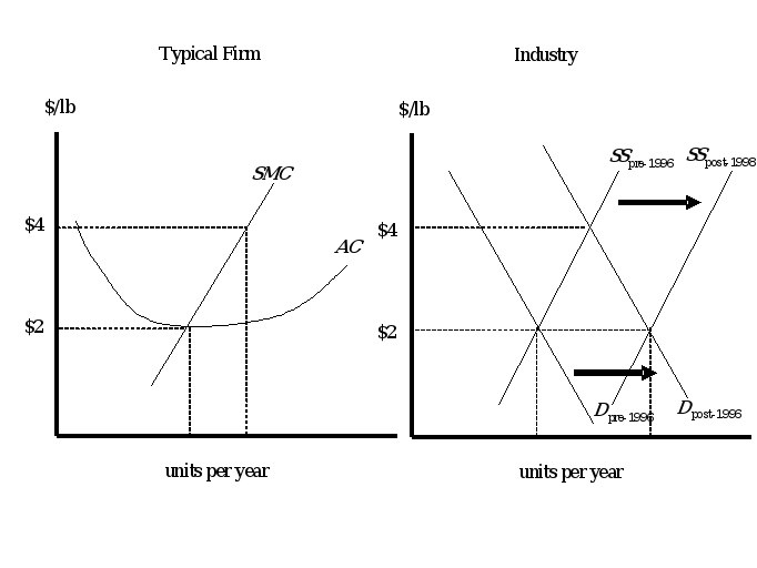
9.26. Suppose that the world market for calcium is perfectly competitive and that, as a first approximation, all existing producers and potential entrants are identical. Consider the following information about the price of calcium:
• Between 1990 and 1995, the market price was stable at about $2 per pound.
• In the first three months of 1996, the market price doubled, reaching a high of $4 per pound, where it remained for the rest of 1996.
• Throughout 1997 and 1998, the market price of calcium declined, eventually reaching $2 per pound by the end of 1998.
• Between 1998 and 2002, the market price was stable at about $2 per pound.
Assuming that the technology for producing calcium did not change between 1990 and 2002 and that input prices faced by calcium producers have remained constant, what explains the pattern of prices that prevailed between 1990 and 2002? Is it likely that there are more producers of calcium in 2002 than there were in 1990? Fewer? The same number? Explain your answer.
The scenario described in the problem can be explained as a constant-cost perfectly competitive industry that experienced an increase in demand (i.e., rightward shift in the demand curve) in early 1996 as shown in the figure below. The price between 1990-1995 reflects a market that is in long-run equilibrium. The increase in price in early 1996 reflects the movement to a short-run equilibrium following the increase in demand. Once price stabilizes at the new short-run equilibrium, firms earn positive economic profits, which attracts new entry. As new entry occurs during 1997 and 1998, the short-run supply curve shifts rightward, causing price to fall. Entry is no longer profitable once price is reestablished at the minimum level of long-run average cost for a typical firm. As a result of the increase in demand, the market now contains more active producers in 2002 than it did in 1990.
9.30. Each firm in the perfectly competitive widget industry produces with the levels of marginal cost (MC) and total variable cost (TVC) at various levels of output Q shown in the following table. Each firm has a total fixed cost of 64 and a sunk fixed cost of 48.
a) Draw a clearly labeled graph of the short-run supply schedule for this firm. Be sure to indicate the shutdown price for each firm and to explain your reasoning for the shape of the supply curve.
b) What is each firm’s producer surplus when the market price is 16?
c) What is the breakeven price for each firm?
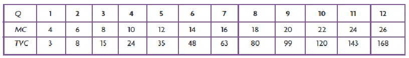
a)
| MC | 10 | 12 | 14 | 16 | 18 | |||
| 15 | 24 | 35 | 48 | 63 | 80 | |||
| Prod surplus =PQ– V - 16 | 4(1)-3 -16 =-15 | 6(2) – 8 - 16 = -12 | 8(3) – 15- 16 = -7 | 10(4) – 24- 16 = 0 | 12(5) – 35 – 16 = 9 | 14(6) – 48 – 16 = 20 | 16(7) – 63-16 =33 | 18(8) – 80 – 16 = 48 |
| Profit = PQ – V – 64 | 4(1) -3 -64 =-63 | 6(2) – 8 - 64 = -60 | 8(3) – 15 - 64 = -55 | 10(4) – 24 - 64 = -48 | 12(5) – 35 - 64 = -39 | 14(6) – 48 - 64 = -28 | 16(7) – 63- 64 = -15 | 18(8) – 80- 64 = 0 |
We know that the supply curve for the firm is just the marginal cost curve for all prices greater than the shut down price. At the shut down price: Producer surplus = Revenue – V – FNonsunk = 0.
FNonsunk = FTotal – FSunk = 64 – 48 = 16.
Simple calculations from the table show that the shut down price is P = 10. If the firm elects to produce when P = 10, it chooses Q so that MC = P, that is, Q = 4.
Producer surplus = Revenue – V – FNonsunk = 10(4) – 24 – 16 = 0.
The graph of the firm’s supply function is as follows. Note that it is the same as the firm’s supply function when P > 10.

b) When P = 16, the firm chooses Q so that MC = P, that is, Q = 7.
Producer surplus = Revenue – V – FNonsunk.
Producer surplus = Revenue – V – FNonsunk = 16(7) – 63 – 16 = 33.
c) Again, calculations from the table show that the breakeven price is P = 18.
When P = 18, the firm chooses Q so that MC = P, that is, Q = 8.
Profit = Revenue – V – FTotal = 18(8) – 80 – 64 = 0.


