Case Problem 3 - "Are You Going to Curve the Grades?"The textbook contains a series of case problems that highlight situations that real organizations could encounter and are related to the weekly lea
Case Problem 3 - "Are You Going to Curve the Grades?"
Course title
Student name
University name
Date
Case Problem 3 - "Are You Going to Curve the Grades?"
Abstract
Grading on a curve will mean several things. Scores in a very Curve take a look at desires changing the numeric cuts to grades assumptive that the take a look at scores virtually statistical distribution. The "curve" during this question is that the "bell curve" in different words statistical distribution curve. the most important activity in wiggly grades is finding the cutoff values, i.e. all-time low potential scores that may receive a D, a C, a B or associate A, severally. The most data you wish from the take a look at scores to line up the curve area unit the mean and variance, in conjunction with some indication that the take a look at scores area unit unremarkably distributed. Note that the whole of the potential take a look at points ne'er comes into the matter. What the cutoff values really area unit depends on what percentages of A's, B's, C's and D's the trainer would love to own. Once you recognize the world below or on top of a definite cutoff worth, then you'll be able to realize the corresponding commonplace score (z-score) that corresponds to the present cutoff worth. The particular cutoff worth is found by standardizing the quality score.
When exam scores are low, students often ask the teacher whether he or she is going to "curve" the grades. The hope is that by curving a low score on the exam, the students will wind up getting a higher letter grade than might otherwise be expected. The term curving grades, or grading on a curve, comes from the bell curve of the normal distribution. If we assume that scores for a large number of students are distributed normally (as with SAT scores) and we also assume that the class average should be a "C," then a teacher might award grades as listed in the table below.
| A | 1.5 standard deviations above the mean or higher |
| B | 0.5 to 1.5 standard deviations above the mean |
| C | Within 0.5 standard deviation of the mean |
| D | 0.5 to 1.5 standard deviations below the mean |
| F | 1.5 standard deviations below the mean or lower |
Suppose a teacher curved grades using the bell curve as in the table above and the grades were indeed normally distributed. What percent of students would get a grade of "A"? Round your answer as a percentage to one decimal place. What percent of students would get a grade of "B"? Round your answer as a percentage to one decimal place. Suggestion: To find the percentage of students getting a grade of "B," subtract the percentage of students 0.5 standard deviations or less above the mean from the percentage of students 1.5 standard deviations or less above the mean.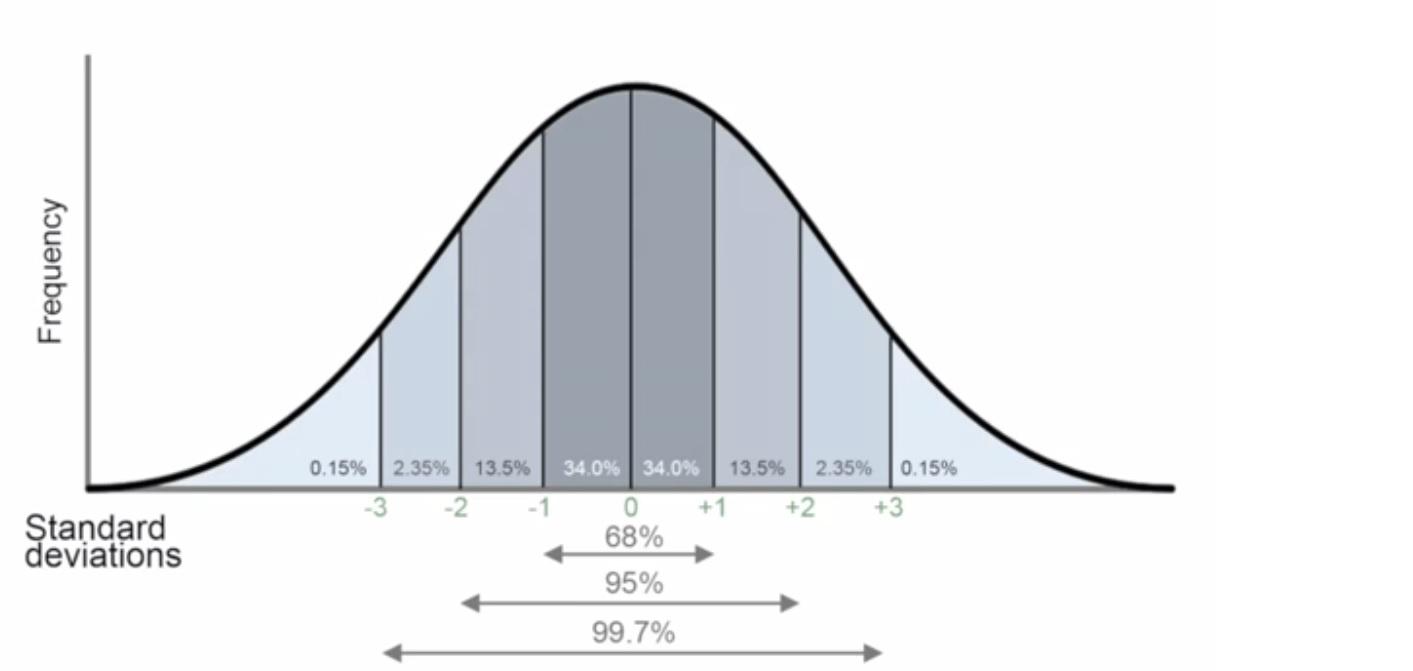
To convert the standard deviations to the percentage of AUC, use a Z-chart or calculator. Using a Z-chart, find the 1.5 and 0.5 Sdvs area values, then subtract to find the area range. The area from 0.5 to 1.5 Sdv is 0.9332 of the area (above 1.5) minus 0.6915 of the area (below 0.5) giving 24.2% of the total area. Here are the percentages for the other deviations. (A) 1.5 standard deviations above the mean or higher (1-0.9332) = 0.0668. 6.7%. (B) 0.5 to 1.5 standard deviations above the mean (0.9332-0.6915) = 0.2417, 24.2%. (C) Within 0.5 standard deviations of the mean (0.6925 - 0.3085) = 0.384. 38.4%. (D) 0.5 to 1.5 standard deviations below the mean (0.3085 - 0.0668) = 0.2417. 24.2 %.( F) 1.5 standard deviations below the mean or lower. (1-0.9332) = 0.0668. 6.7%
Conclusion
The standard deviation tells you how big a gap between raw scores is significant. Thus if 70 is the mean or average, and 20 is the standard deviation, then 90 is meaningfully different from 70. 75 is less significantly different from 70—or to be more precise, you cannot be as sure that the difference is not random. So if you then decide that since 70 was the average, that might say a B. 90 could then be A, because you know that the difference is significant, 50 would be a C, etc. So besides 70, you’d have zero, besides 80, you’d have 0.5, besides 90, you’d have 1.0, etc. Some people will then be upset that there are no D’s, for instance. But this method tells you (more reliably for more scores) how significant the difference in performance between one student and another is.
References
Mendenhall, W., Beaver, R. J., & Beaver, B. M. (2012). Introduction to probability and statistics. Cengage Learning.
Solutioninncom. (2018). Solutioninncom. Retrieved 25 May, 2018, from https://www.solutioninn.com/very-often-at-the-end-of-an-exam-that-seemed
Southeasternedu. (2018). Southeasternedu. Retrieved 25 May, 2018, from https://www2.southeastern.edu/Academics/Faculty/dgurney/Math241/StatTopics/GradeCurves.htm


