Can anyone help with 2 assignments due by midnight U.S. Mountain time. See attached file. thank you.
Exercise 26
Graded Questions:
1. Plot the frequency distribution for “Age at Enrollment” by hand or by using SPSS.
2. How would you characterize the skewness of the distribution in Question 1—positively skewed,
negatively skewed, or approximately normal? Provide a rationale for your answer.
3. Compare the original skewness statistic and Shapiro-Wilk statistic with those of the smaller
dataset ( n = 15) for the variable “Age at First Arrest.” How did the statistics change, and how
would you explain these differences?
4. Plot the frequency distribution for “Years of Education” by hand or by using SPSS.
5. How would you characterize the kurtosis of the distribution in Question 4—leptokurtic, mesokurtic,
or platykurtic? Provide a rationale for your answer.
6. What is the skewness statistic for “Age at Enrollment”? How would you characterize the magnitude
of the skewness statistic for “Age at Enrollment”?
7. What is the kurtosis statistic for “Years of Education”? How would you characterize the magnitude
of the kurtosis statistic for “Years of Education”?
8. Using SPSS, compute the Shapiro-Wilk statistic for “Number of Times Fired from Job.” What
would you conclude from the results?
9. In the SPSS output table titled “Tests of Normality,” the Shapiro-Wilk statistic is reported along
with the Kolmogorov-Smirnov statistic. Why is the Kolmogorov-Smirnov statistic inappropriate
to report for these example data?
10. How would you explain the skewness statistic for a particular frequency distribution being low
and the Shapiro-Wilk statistic still being signifi cant at p < 0.05?
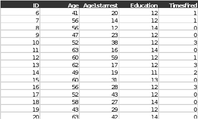
Data Set for Question 26:
Exercise 10
STATISTICAL TECHNIQUE IN REVIEW
Most research reports describe the subjects or participants who comprise the study
sample. This description of the sample is called the sample characteristics , which may
be presented in a table and/or the narrative of the article. The sample characteristics are
often presented for each of the groups in a study (i.e., intervention and control groups).
Descriptive statistics are calculated to generate sample characteristics, and the type of
statistic conducted depends on the level of measurement of the demographic variables
included in a study ( Grove, Burns, & Gray, 2013 ). For example, data collected on gender
is nominal level and can be described using frequencies, percentages, and mode. Measuring
educational level usually produces ordinal data that can be described using frequencies,
percentages, mode, median, and range. Obtaining each subject ’ s specifi c age is an
example of ratio data that can be described using mean, range, and standard deviation.
Interval and ratio data are analyzed with the same statistical techniques and are sometimes
referred to as interval/ratio-level data in this text.
RESEARCH ARTICLE
Source
Oh, E. G., Yoo, J. Y., Lee, J. E., Hyun, S. S., Ko, I. S., & Chu, S. H. (2014). Effects of a threemonth
therapeutic lifestyle modifi cation program to improve bone health in postmenopausal
Korean women in a rural community: A randomized controlled trial. Research in
Nursing & Health, 37 (4), 292–301.
Introduction
Oh and colleagues (2014) conducted a randomized controlled trial (RCT) to examine the
effects of a therapeutic lifestyle modifi cation (TLM) intervention on the knowledge, selfeffi
cacy, and behaviors related to bone health in postmenopausal women in a rural community.
The study was conducted using a pretest-posttest control group design with a
sample of 41 women randomly assigned to either the intervention ( n = 21) or control
group ( n = 20). “The intervention group completed a 12-week, 24-session TLM program
of individualized health monitoring, group health education, exercise, and calcium–
vitamin D supplementation. Compared with the control group, the intervention group
showed signifi cant increases in knowledge and self-effi cacy and improvement in diet and
exercise after 12 weeks, providing evidence that a comprehensive TLM program can be
effective in improving health behaviors to maintain bone health in women at high risk
of osteoporosis” ( Oh et al., 2014 , p. 292).
EXERCISE
10
Relevant Study Results
“Bone mineral density (BMD; g/cm 2 ) was measured by dual energy x-ray absorptiometry
(DXA) with the use of a DEXXUM T machine . . . . A daily calibration inspection was performed.
The error rate for these scans is less than 1%. Based on the BMD data, the participants
were classifi ed into three groups: osteoporosis (a BMD T -score less than − 2.5);
osteopenia (a BMD T -score between − 2.5 and − 1.0); and normal bone density (a BMD
T -score higher than − 1.0)” ( Oh et al. 2014 , p. 295).
“Characteristics of Participants
The study participants were 51–83 years old, and the mean age was 66.2 years ( SD = 8.2).
The mean BMI was 23.8 kg/m 2 ( SD = 3.2). Most participants did not consume alcoholic
drinks, and all were nonsmokers. Antihypertensives and analgesics such as aspirin and
acetaminophen were the most common medications taken by the participants. Less than
20% of participants had a regular routine of exercise at least three times per week. Daily
calcium- and vitamin D-rich food intake (e.g., dairy products, fi sh oil, meat, and eggs) was
low. Seventy-fi ve percent ( n = 31) of the participants had osteoporosis or osteopenia.
There were no differences in the baseline characteristics of the groups ( Table 2 ). The
adherence rate to the TLM program was 99.6%” ( Oh et al., 2014 , p. 296).
TABLE 2 BASELINE CHARACTERISTICS AND HOMOGENEITY OF THE TREATMENT AND
CONTROL GROUPS
Intervention ( n = 21) Control ( n = 20)
Characteristic Mean ± SD Mean ± SD t or χ 2 a
Anthropometric
Age (years) 65.95 ± 8.59 66.35 ± 7.94 0.154
Height (cm) 152.33 ± 6.53 150.57 ± 6.01 0.896
Weight (kg) 57.90 ± 10.85 54.66 ± 9.48 1.016
BMI (kg/m 2 ) 24.17 ± 3.14 23.38 ± 3.32 0.782
Lifestyle
Years since menopause 20.21 ± 10.44 17.5 ± 11.05 0.767
Calcium-rich food intake (times/week) 27.3 ± 11.4 23.8 ± 8.8 1.110
Vitamin D-rich food intake (times/week) 2.4 ± 2.5 3.1 ± 3.1 0.705
Intervention ( n = 21) Control ( n = 20)
Characteristic n % n % t or χ 2 a
History of fracture 8 38 5 25 1.026
Regular exercise ( ≥ 3 times/week) 4 19 4 20 0.006
Non-drinker (alcohol) 20 95 20 100 0.024
Non-smoker 21 100 20 100 0.024
Bone status b
Normal (T ≥ − 1.0) 6 29 4 20 1.995
Osteopenia ( − 1.0 > T > − 2.5) 8 38 12 60
Osteoporosis (T ≤ − 2.5) 7 33 4 20
Intervention ( n = 21) Control ( n = 20)
Characteristic Mean ± SD Mean ± SD t or χ 2 a
BMD
Lumbar 2–4 0.83 ± 0.12 0.85 ± 0.20 0.526
Femur neck 0.67 ± 0.15 0.67 ± 0.13 0.055
Bone biomarkers
Serum osteocalcin (ng/ml) 13.97 ± 4.90 15.85 ± 5.64 1.135
Serum calcium (mg/dl) 9.47 ± 0.40 9.54 ± 0.59 0.405
Serum phosphorus (mg/dl) 3.68 ± 0.44 3.70 ± 0.50 0.165
Serum alkaline phosphatase (IU/L) 68.43 ± 21.52 66.70 ± 13.24 0.308
Serum 25-OH-Vitamin D (ng/ml) 14.03 ± 4.34 12.38 ± 4.65 1.177
Urine deoxypyridinoline (nM/mM creatinine) 5.70 ± 1.70 5.95 ± 1.12 0.555
Note. SD, standard deviation; BMD, bone mineral density (g/cm 2 ).
a All group differences p > 0.05.
b Defi ned from T -score of femur neck site based on World Health Organization criteria.
Oh, E. G., Yoo, J. Y., Lee, J. E., Hyun, S. S., Ko, I. S., & Chu, S. H. (2014). Effects of a three-month therapeutic lifestyle modifi cation
program to improve bone health in postmenopausal Korean women in a rural community: A randomized controlled trial. Research in
Exercise 10 graded questions:
1. What demographic variables were measured at the nominal level of measurement in the Oh et al.
(2014) study? Provide a rationale for your answer.
2. What statistics were calculated to describe body mass index (BMI) in this study? Were these
appropriate? Provide a rationale for your answer.
3. Were the distributions of scores for BMI similar for the intervention and control groups? Provide
a rationale for your answer.
4. Was there a signifi cant difference in BMI between the intervention and control groups? Provide
a rationale for your answer.
5. Based on the sample size of N = 41, what frequency and percentage of the sample smoked? What
frequency and percentage of the sample were non-drinkers (alcohol)? Show your calculations
and round to the nearest whole percent.
6. What measurement method was used to measure the bone mineral density (BMD) for the study
participants? Discuss the quality of this measurement method and document your response.
7. What statistic was calculated to determine differences between the intervention and control
groups for the lumbar and femur neck BMDs? Were the groups signifi cantly different for BMDs?
8. The researchers stated that there were no signifi cant differences in the baseline characteristics
of the intervention and control groups (see Table 2 ). Are these groups heterogeneous or homogeneous
at the beginning of the study? Why is this important in testing the effectiveness of the
therapeutic lifestyle modifi cation (TLM) program?
9. Oh et al. (2014 , p. 296) stated that “the adherence rate to the TLM program was 99.6%.” Discuss
the importance of intervention adherence, and document your response.
10. Was the sample for this study adequately described? Provide a rationale for your answer.


