Looking fo help please with Four chapters questions.

Chapter 27 Questions to be graded

1. What is the mean age of the sample data?

2. What percentage of patients never used tobacco?

3. What is the standard deviation for age?

4. Are there outliers among the values of age? Provide a rationale for your answer.

5. What is the range of age values?

6. What percentage of patients were taking infliximab?

7. What percentage of patients had rheumatoid arthritis as their primary diagnosis?

8. What percentage of patients had irritable bowel syndrome as their primary diagnosis?

9. What is the 95% CI for age?

10. What percentage of patients had psoriatic arthritis as their primary diagnosis?

There are two major classes of statistics: descriptive statistics and inferential statistics.

Descriptive statistics are computed to reveal characteristics of the sample data set and to

describe study variables. Inferential statistics are computed to gain information about

effects and associations in the population being studied. For some types of studies,

descriptive statistics will be the only approach to analysis of the data. For other studies,

descriptive statistics are the fi rst step in the data analysis process, to be followed by inferential

statistics. For all studies that involve numerical data, descriptive statistics are

crucial in understanding the fundamental properties of the variables being studied. Exercise

27 focuses only on descriptive statistics and will illustrate the most common descriptive

statistics computed in nursing research and provide examples using actual clinical

data from empirical publications.

MEASURES OF CENTRAL TENDENCY

A measure of central tendency is a statistic that represents the center or middle of a

frequency distribution. The three measures of central tendency commonly used in nursing

research are the mode, median ( MD ), and mean ( X ). The mean is the arithmetic average

of all of a variable ’ s values. The median is the exact middle value (or the average of the

middle two values if there is an even number of observations). The mode is the most

commonly occurring value or values (see Exercise 8 ).

The following data have been collected from veterans with rheumatoid arthritis ( Tran,

Hooker, Cipher, & Reimold, 2009 ). The values in Table 27-1 were extracted from a larger

sample of veterans who had a history of biologic medication use (e.g., infl iximab [Remicade],

etanercept [Enbrel]). Table 27-1 contains data collected from 10 veterans who had

stopped taking biologic medications, and the variable represents the number of years that

each veteran had taken the medication before stopping.

Because the number of study subjects represented below is 10, the correct statistical

notation to refl ect that number is:

n 10

Note that the n is lowercase, because we are referring to a sample of veterans. If the

data being presented represented the entire population of veterans, the correct notation

is the uppercase N. Because most nursing research is conducted using samples, not populations,

all formulas in the subsequent exercises will incorporate the sample notation, n.

Mode

The mode is the numerical value or score that occurs with the greatest frequency; it does

not necessarily indicate the center of the data set. The data in Table 27-1 contain two

EXERCISE

292 EXERCISE 27 • Calculating Descriptive Statistics

modes: 1.5 and 3.0. Each of these numbers occurred twice in the data set. When two

modes exist, the data set is referred to as bimodal ; a data set that contains more than

two modes would be multimodal .

Median

The median ( MD ) is the score at the exact center of the ungrouped frequency distribution.

It is the 50th percentile. To obtain the MD , sort the values from lowest to highest. If the

number of values is an uneven number, exactly 50% of the values are above the MD and

50% are below it. If the number of values is an even number, the MD is the average of the

two middle values. Thus the MD may not be an actual value in the data set. For example,

the data in Table 27-1 consist of 10 observations, and therefore the MD is calculated as

the average of the two middle values.

MD 

1 5 2 0

1 75

. .

Mean

The most commonly reported measure of central tendency is the mean. The mean is the

sum of the scores divided by the number of scores being summed. Thus like the MD, the

mean may not be a member of the data set. The formula for calculating the mean is as

follows:



where

X = mean

Σ = sigma, the statistical symbol for summation

X = a single value in the sample

n = total number of values in the sample

The mean number of years that the veterans used a biologic medication is calculated

as follows:

X 

0 1 0 3 1 3 1 5 1 5 2 0 2 2 3 0 3 0 4 0

1 9

. . . . . . . . . .

. years

EXERCISE 27 • Calculating Descriptive Statistics

Descriptives

Statistic Std. Error

Duration of Biologic Use

1.890 .3860

Lower Bound 1.017

Upper Bound 2.763

1.872

1.750

1.490

1.2206

4.0

3.9

2.0

.159 .687

-.437 1.334

Mean

95% Confidence Interval for Mean

5% Trimmed Mean

Median

Variance

Std. Deviation

Minimum

Maximum

Range

Interquartile Range

Skewness

Kurtosis

The second set of output (from the second set of SPSS commands in Step 2) contains the

descriptive statistics for “Duration,” including the mean, s (standard deviation), SE , 95%

confi dence interval for the mean, median, variance, minimum value, maximum value,

range, and skewness and kurtosis statistics. As shown in the output, mean number of

years for duration is 1.89, and the SD is 1.22. The 95% CI is 1.02–2.76.

SPSS COMPUTATIONS

A retrospective descriptive study examined the duration of biologic use from veterans

with rheumatoid arthritis ( Tran et al., 2009 ). The values in Table 27-4 were extracted from

a larger sample of veterans who had a history of biologic medication use (e.g., infl iximab

[Remicade], etanercept [Enbrel]). Table 27-4 contains simulated demographic data collected

from 10 veterans who had stopped taking biologic medications. Age at study enrollment,

duration of biologic use, race/ethnicity, gender (F = female), tobacco use (F = former

use, C = current use, N = never used), primary diagnosis (3 = irritable bowel syndrome, 4

= psoriatic arthritis, 5 = rheumatoid arthritis, 6 = reactive arthritis), and type of biologic

medication used were among the study variables examined.

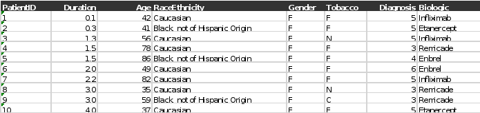
TABLE 27-4 DEMOGRAPHIC VARIABLES OF VETERANS WITH RHEUMATOID ARTHRITIS

Patient ID/Duration/(yrs) /Age Race or Ethnicity /Gender /Tobacco/ Diagnosis /Biologic

1.) 0.1 /42 /Caucasian/ F /F/ 5 /Infliximab

2.) 0.3 /41 /Black, not of Hispanic Origin/ F/ F/ 5 /Etanercept

3.) 1.3 /56/ Caucasian /F /N /5/ Infliximab

4.) 1.5/ 78/ Caucasian/ F/ F /3 /Infliximab

5.) 1.5 /86 /Black, not of Hispanic Origin/ F/ F/ 4/ Etanercept

6.) 2.0/ 49/ Caucasian /F /F/ 6/ Etanercept

7.)2.2/ 82/ Caucasian/ F/ F/ 5 /Infliximab

8.) 3.0/ 35/ Caucasian /F/ N /3 /Infliximab

9.) 3.0 /59/ Black, not of Hispanic Origin/ F/ C/ 3/ Infliximab

10.) 4.0 /37/ Caucasian/ F /F/ 5/ Etanercept

Data set Exercise 27:

Looking fo help please with Four chapters questions. 1

Chapter 6 Questions to be graded:

1. What are the frequency and percentage of the COPD patients in the severe airfl ow limitation

group who are employed in the Eckerblad et al. (2014) study?

2. What percentage of the total sample is retired? What percentage of the total sample is on sick

leave?

3. What is the total sample size of this study? What frequency and percentage of the total sample

were still employed? Show your calculations and round your answer to the nearest whole percent.

4. What is the total percentage of the sample with a smoking history—either still smoking or former

smokers? Is the smoking history for study participants clinically important? Provide a rationale

for your answer.

5. What are pack years of smoking? Is there a significant difference between the moderate and severe

airflow limitation groups regarding pack years of smoking? Provide a rationale for your answer.

6. What were the four most common psychological symptoms reported by this sample of patients

with COPD? What percentage of these subjects experienced these symptoms? Was there a significant difference between the moderate and severe airflow limitation groups for psychological

symptoms?

7. What frequency and percentage of the total sample used short-acting β2 -agonists? Show your

calculations and round to the nearest whole percent.

8. Is there a significant difference between the moderate and severe airflow limitation groups

regarding the use of short-acting β 2 -agonists? Provide a rationale for your answer.

9. Was the percentage of COPD patients with moderate and severe airflow limitation using short acting

β 2 -agonists what you expected? Provide a rationale with documentation for your answer.

10. Are these findings ready for use in practice? Provide a rationale for your answer.

STATISTICAL TECHNIQUE IN REVIEW

Frequency is the number of times a score or value for a variable occurs in a set of data.

Frequency distribution is a statistical procedure that involves listing all the possible

values or scores for a variable in a study. Frequency distributions are used to organize

study data for a detailed examination to help determine the presence of errors in coding

or computer programming ( Grove, Burns, & Gray, 2013 ). In addition, frequencies and

percentages are used to describe demographic and study variables measured at the nominal

or ordinal levels.

Percentage can be defi ned as a portion or part of the whole or a named amount in

every hundred measures. For example, a sample of 100 subjects might include 40 females

and 60 males. In this example, the whole is the sample of 100 subjects, and gender is

described as including two parts, 40 females and 60 males. A percentage is calculated

by dividing the smaller number, which would be a part of the whole, by the larger

number, which represents the whole. The result of this calculation is then multiplied

by 100%. For example, if 14 nurses out of a total of 62 are working on a given day, you

can divide 14 by 62 and multiply by 100% to calculate the percentage of nurses working

that day. Calculations: (14 ÷ 62) × 100% = 0.2258 × 100% = 22.58% = 22.6%. The answer

also might be expressed as a whole percentage, which would be 23% in this example.

A cumulative percentage distribution involves the summing of percentages from the

top of a table to the bottom. Therefore the bottom category has a cumulative percentage

of 100% (Grove, Gray, & Burns, 2015). Cumulative percentages can also be used to determine

percentile ranks, especially when discussing standardized scores. For example, if 75%

of a group scored equal to or lower than a particular examinee ’ s score, then that examinee ’ s

rank is at the 75 th percentile. When reported as a percentile rank, the percentage is often

rounded to the nearest whole number. Percentile ranks can be used to analyze ordinal

data that can be assigned to categories that can be ranked. Percentile ranks and cumulative

percentages might also be used in any frequency distribution where subjects have only one

value for a variable. For example, demographic characteristics are usually reported with the

frequency ( f ) or number ( n ) of subjects and percentage (%) of subjects for each level of a

demographic variable. Income level is presented as an example for 200 subjects:

Income Level Frequency ( f ) Percentage (%) Cumulative %

1. < $40,000 20 10% 10%

2. $40,000–$59,999 50 25% 35%

3. $60,000–$79,999 80 40% 75%

4. $80,000–$100,000 40 20% 95%

5. > $100,000 10 5% 100%

EXERCISE

60 EXERCISE 6 • Understanding Frequencies and Percentages

In data analysis, percentage distributions can be used to compare fi ndings from different

studies that have different sample sizes, and these distributions are usually arranged in

tables in order either from greatest to least or least to greatest percentages ( Plichta &

Kelvin, 2013 ).

RESEARCH ARTICLE

Source

Eckerblad, J., Tödt, K., Jakobsson, P., Unosson, M., Skargren, E., Kentsson, M., & Theander,

K. (2014). Symptom burden in stable COPD patients with moderate to severe airfl ow

limitation. Heart & Lung, 43 (4), 351–357.

Introduction

Eckerblad and colleagues (2014 , p. 351) conducted a comparative descriptive study to

examine the symptoms of “patients with stable chronic obstructive pulmonary disease

(COPD) and determine whether symptom experience differed between patients with moderate

or severe airfl ow limitations.” The Memorial Symptom Assessment Scale (MSAS)

was used to measure the symptoms of 42 outpatients with moderate airfl ow limitations

and 49 patients with severe airfl ow limitations. The results indicated that the mean

number of symptoms was 7.9 ( } 4.3) for both groups combined, with no signifi cant differences

found in symptoms between the patients with moderate and severe airfl ow limitations.

For patients with the highest MSAS symptom burden scores in both the moderate

and the severe limitations groups, the symptoms most frequently experienced included

shortness of breath, dry mouth, cough, sleep problems, and lack of energy. The researchers

concluded that patients with moderate or severe airfl ow limitations experienced multiple

severe symptoms that caused high levels of distress. Quality assessment of COPD

patients ’ physical and psychological symptoms is needed to improve the management of

their symptoms.

Relevant Study Results

Eckerblad et al. (2014 , p. 353) noted in their research report that “In total, 91 patients

assessed with MSAS met the criteria for moderate ( n = 42) or severe airfl ow limitations

( n = 49). Of those 91 patients, 47% were men, and 53% were women, with a mean age of

68 ( } 7) years for men and 67 ( } 8) years for women. The majority (70%) of patients were

married or cohabitating. In addition, 61% were retired, and 15% were on sick leave.

Twenty-eight percent of the patients still smoked, and 69% had stopped smoking. The

mean BMI (kg/m 2 ) was 26.8 ( } 5.7).

There were no signifi cant differences in demographic characteristics, smoking history,

or BMI between patients with moderate and severe airfl ow limitations ( Table 1 ). A lower

proportion of patients with moderate airfl ow limitation used inhalation treatment with

glucocorticosteroids, long-acting β 2 -agonists and short-acting β 2 -agonists, but a higher

proportion used analgesics compared with patients with severe airfl ow limitation.

Symptom prevalence and symptom experience

The patients reported multiple symptoms with a mean number of 7.9 ( } 4.3) symptoms

(median = 7, range 0–32) for the total sample, 8.1 ( } 4.4) for moderate airfl ow limitation

and 7.7 ( } 4.3) for severe airfl ow limitation ( p = 0.36) . . . . Highly prevalent physical symptoms

( ≥ 50% of the total sample) were shortness of breath (90%), cough (65%), dry mouth

(65%), and lack of energy (55%). Five additional physical symptoms, feeling drowsy, pain,

Understanding Frequencies and Percentages • EXERCISE 6 61

TABLE 1 BACKGROUND CHARACTERISTICS AND USE OF MEDICATION FOR PATIENTS WITH

STABLE CHRONIC OBSTRUCTIVE LUNG DISEASE CLASSIFIED IN PATIENTS WITH

MODERATE AND SEVERE AIRFLOW LIMITATION

Moderate

n = 42

Severe

n = 49 p Value

Sex, n (%) 0.607

Women 19 (45) 29 (59)

Men 23 (55) 20 (41)

Age (yrs), mean ( SD ) 66.5 (8.6) 67.9 (6.8) 0.396

Married/cohabitant n (%) 29 (69) 34 (71) 0.854

Employed, n (%) 7 (17) 7 (14) 0.754

Smoking, n % 0.789

Smoking 13 (31) 12 (24)

Former smokers 28 (67) 35 (71)

Never smokers 1 (2) 2 (4)

Pack years smoking, mean ( SD ) 29.1 (13.5) 34.0 (19.5) 0.177

BMI (kg/m 2 ), mean ( SD ) 27.2 (5.2) 26.5 (6.1) 0.555

FEV 1 % of predicted, mean ( SD ) 61.6 (8.4) 42.2 (5.8) < 0.001

SpO 2 % mean ( SD ) 95.8 (2.4) 94.5 (3.0) 0.009

Physical health, mean ( SD ) 3.2 (0.8) 3.0 (0.8) 0.120

Mental health, mean ( SD ) 3.7 (0.9) 3.6 (1.0) 0.628

Exacerbation previous 6 months, n (%) 14 (33) 15 (31) 0.781

Admitted to hospital previous year, n (%) 10 (24) 14 (29) 0.607

Medication use, n (%)

Inhaled glucocorticosteroids 30 (71) 44 (90) 0.025

Systemic glucocorticosteroids 3 (6.3) 0 (0) 0.094

Anticholinergic 32 (76) 42 (86) 0.245

Long-acting β 2 -agonists 30 (71) 45 (92) 0.011

Short-acting β 2 -agonists 13 (31) 32 (65) 0.001

Analgesics 11 (26) 5 (10) 0.046

Statins 8 (19) 11 (23) 0.691

Eckerblad, J., Tödt, K., Jakobsson, P., Unosson, M., Skargren, E., Kentsson, M., & Theander, K. (2014). Symptom burden in stable

COPD patients with moderate to severe airfl ow limitation. Heart & Lung, 43 (4), p. 353.

numbness/tingling in hands/feet, feeling irritable, and dizziness, were reported by between

25% and 50% of the patients. The most commonly reported psychological symptom was

diffi culty sleeping (52%), followed by worrying (33%), feeling irritable (28%) and feeling

sad (22%). There were no signifi cant differences in the occurrence of physical and psychological

symptoms between patients with moderate and severe airfl ow limitations”

( Eckerblad et al., 2014 , p. 353).

62 EXERCISE 6 • Understanding Frequencies and Percentages

Exercise 8 Questions to be graded:

1. The number of nursing students enrolled in a particular nursing program between the years of

2010 and 2016, respectively, were 563, 593, 606, 520, 563, 610, and 577. Determine the mean

( X ), median ( MD ), and mode of the number of the nursing students enrolled in this program.

Show your calculations.

2. What is the mode for the variable inpatient complications in Table 2 of the Winkler et al. (2014)

study? What percentage of the study participants had this complication?

3. Does the distribution of inpatient complications have a single mode, or is this distribution

bimodal or multimodal? Provide a rationale for your answer.

4. As reported in Table 1 , what are the three most common cardiovascular medical history events

in this study, and why is it clinically important to know the frequency of these events?

5. What are the mean and median lengths of stay (LOS) for the study participants?

6. Are the mean and median for LOS similar or different? What might this indicate about the

distribution of the sample? Provide a rationale for your answer.

7. Examine the study results and determine the mode for arrhythmias experienced by the participants.

What was the second most common arrhythmia in this sample?

8. Was the most common arrhythmia in Question 7 related to LOS? Was this result statistically

signifi cant? Provide a rationale for your answer.

9. What study variables were independently predictive of the 50 premature ventricular contractions

(PVCs) per hour in this study?

10. In Table 1 , what race is the mode for this sample? Should these study fi ndings be generalized to

American Indians with ACS? Provide a rationale for your answer.

STATISTICAL TECHNIQUE IN REVIEW

Mean, median, and mode are the three measures of central tendency used to describe

study variables. These statistical techniques are calculated to determine the center of a

distribution of data, and the central tendency that is calculated is determined by the level

of measurement of the data (nominal, ordinal, interval, or ratio; see Exercise 1 ). The mode

is a category or score that occurs with the greatest frequency in a distribution of scores

in a data set. The mode is the only acceptable measure of central tendency for analyzing

nominal-level data, which are not continuous and cannot be ranked, compared, or subjected

to mathematical operations. If a distribution has two scores that occur more frequently

than others (two modes), the distribution is called bimodal . A distribution with

more than two modes is multimodal ( Grove, Burns, & Gray, 2013 ).

The median ( MD ) is a score that lies in the middle of a rank-ordered list of values of

a distribution. If a distribution consists of an odd number of scores, the MD is the middle

score that divides the rest of the distribution into two equal parts, with half of the values

falling above the middle score and half of the values falling below this score. In a distribution

with an even number of scores, the MD is half of the sum of the two middle numbers

of that distribution. If several scores in a distribution are of the same value, then the MD

will be the value of the middle score. The MD is the most precise measure of central tendency

for ordinal-level data and for nonnormally distributed or skewed interval- or ratiolevel

data. The following formula can be used to calculate a median in a distribution of

scores.

Median(MD) (N 1) 2

N is the number of scores

Example: N Median th score 31

31 1

32 2 16

Example: N Median . th score 40

40 1

41 2 20 5

Thus in the second example, the median is halfway between the 20 th and the 21 st scores.

The mean ( X ) is the arithmetic average of all scores of a sample, that is, the sum of its

individual scores divided by the total number of scores. The mean is the most accurate

measure of central tendency for normally distributed data measured at the interval and

ratio levels and is only appropriate for these levels of data (Grove, Gray, & Burns, 2015).

In a normal distribution, the mean, median, and mode are essentially equal (see Exercise

26 for determining the normality of a distribution). The mean is sensitive to extreme

80 EXERCISE 8 • Measures of Central Tendency: Mean, Median, and Mode

scores such as outliers. An outlier is a value in a sample data set that is unusually low or

unusually high in the context of the rest of the sample data. If a study has outliers, the

mean is most affected by these, so the median might be the measure of central tendency

included in the research report ( Plichta & Kelvin, 2013 ). The formula for the mean is:

MeanX

Σ X is the sum of the raw scores in a study

N is the sample size or number of scores in the study

Example:Raw scores 8, 9, 9,10,11,11 N 6 Mean 58 6 9.666 9.67

RESEARCH ARTICLE

Source

Winkler, C., Funk, M., Schindler, D. M., Hemsey, J. Z., Lampert, R., & Drew, B. J. (2013).

Arrhythmias in patients with acute coronary syndrome in the fi rst 24 hours of hospitalization.

Heart & Lung, 42 (6), 422–427.

Introduction

Winkler and colleagues (2013) conducted their study to describe the arrhythmias of a

population of patients with acute coronary syndrome (ACS) during their fi rst 24 hours

of hospitalization and to explore the link between arrhythmias and patients ’ outcomes.

The patients with ACS were admitted through the emergency department (ED), where a

Holter recorder was attached for continuous 12-lead electrocardiographic (ECG) monitoring.

The ECG data from the Holter recordings of 278 patients with ACS were analyzed.

The researchers found that “approximately 22% of patients had more than 50 premature

ventricular contractions (PVCs) per hour. Non-sustained ventricular tachycardia (VT)

occurred in 15% of the patients . . . . Only more than 50 PVCs/hour independently predicted

an increased length of stay ( p < 0.0001). No arrhythmias predicted mortality. Age

greater than 65 years and a fi nal diagnosis of acute myocardial infarction (AMI) independently

predicted more than 50 PVCs per hour ( p = 0.0004)” ( Winkler et al., 2013 , p. 422).

Winkler and colleagues (2013 , p. 426) concluded: “Life-threatening arrhythmias are

rare in patients with ACS, but almost one quarter of the sample experienced isolated

PVCs. There was a signifi cant independent association between PVCs and a longer length

of stay (LOS), but PVCs were not related to other adverse outcomes. Rapid treatment of

the underlying ACS should remain the focus, rather than extended monitoring for

arrhythmias we no longer treat.”

Relevant Study Results

The demographic and clinical characteristics of the sample and the patient outcomes for

this study are presented in this exercise. “The majority of the patients ( n = 229; 83%) had

a near complete Holter recording of at least 20 h and 171 (62%) had a full 24 h recorded.

We included recordings of all patients in the analysis. The mean duration of continuous

12-lead Holter recording was 21 } 6 (median 24) h.

The mean patient age was 66 years and half of the patients identifi ed White as

their race ( Table 1 ). There were more males than females and most patients (92%) experienced

chest pain as one of the presenting symptoms to the ED. Over half of the patients

Measures of Central Tendency: Mean, Median, and Mode • EXERCISE 8 81

TABLE 1 DEMOGRAPHIC AND CLINICAL CHARACTERISTICS OF THE SAMPLE ( N = 278)

Characteristic N %

Gender

Male 158 57

Female 120 43

Race

White 143 51

Asian 60 22

Black 50 18

American Indian 23 8

Pacifi c Islander 2 < 1

Presenting Symptoms to the ED (May Have > 1)

Chest pain 255 92

Shortness of breath 189 68

Jaw, neck, arm, or back pain 152 55

Diaphoresis 116 42

Nausea and vomiting 96 35

Syncope 11 4

Cardiovascular Risk Factors (May Have > 1)

Hypertension 211 76

Hypercholesterolemia 175 63

Family history of CAD 148 53

Diabetes 81 29

Smoking (current) 56 20

Cardiovascular Medical History (May Have > 1)

Personal history of CAD 176 63

History of unstable angina 124 45

Previous acute myocardial infarction 114 41

Previous percutaneous coronary intervention 85 31

Previous CABG surgery 54 19

History of arrhythmias 53 19

Final Diagnosis

Unstable angina 180 65

Non-ST elevation myocardial infarction 74 27

ST elevation myocardial infarction 24 9

Interventions during 24-h Holter Recording

PCI ≤ 90 min of ED admission 14 5

PCI > 90 min of ED admission 3 1

Thrombolytic medication 3 1

Interventions Any Time during Hospitalization

PCI 76 27

Treated with anti-arrhythmic medication 16 6

CABG surgery 22 8

Mean ( SD ) Median Range

Age (years) 66 (14) 66 30–102

ECG recording time (hours) 21 (6) 24 2–25

ED, emergency department; CAD, coronary artery disease; CABG, coronary artery bypass graft; PCI, percutaneous coronary

intervention; SD , standard deviation; ECG, electrocardiogram.

Winkler, C., Funk, M., Schindler, D. M., Hemsey, J. Z., Lampert, R., & Drew, B. J. (2013). Arrhythmias in patients with acute

coronary syndrome in the fi rst 24 hours of hospitalization. Heart & Lung, 42 (6), p. 424

experienced shortness of breath (68%) and jaw, neck, arm, or back pain (55%). Hypertension

was the most frequently occurring cardiovascular risk factor (76%), followed by

hypercholesterolemia (63%) and family history of coronary artery disease (53%). A majority

had a personal history of coronary artery disease (63%) and 19% had a history of

arrhythmias” ( Winkler et al., 2013 , pp. 423–424).

Winkler et al. (2013 , p. 424) also reported: “We categorized patient outcomes into four

groups: 1) inpatient complications (of which some patients may have experienced more

than one); 2) inpatient length of stay; 3) readmission to either the ED or the hospital

within 30-days and 1-year of initial hospitalization; and 4) death during hospitalization,

within 30-days, and 1-year after discharge ( Table 2 ). These are outcomes that are reported

in many contemporary studies of patients with ACS. Thirty-two patients (11.5%) were lost

to 1-year follow-up, resulting in a sample size for the analysis of 1-year outcomes of 246

patients” ( Winkler et al., 2013 , p. 424).

TABLE 2 OUTCOMES DURING INPATIENT STAY, AND WITHIN 30 DAYS AND 1 YEAR OFHOSPITALIZATION ( N = 278)

Outcomes N %

Inpatient complications (may have > 1)

AMI post admission for patients admitted with UA 21 8

Transfer to intensive care unit 17 6

Cardiac arrest 7 3

AMI extension (detected by 2nd rise in CK-MB) 6 2

Cardiogenic shock 5 2

New severe heart failure/pulmonary edema 2 1

Readmission *

30-day

To ED for a cardiovascular reason 42 15

To hospital for ACS 13 5

1-year ( N = 246)

To ED for a cardiovascular reason 108 44

To hospital for ACS 24 10

All-cause mortality †

Inpatient 10 4

30-day 13 5

1-year ( N = 246) 27 11

Mean ( SD ) Median Range

Length of stay (days) 5.37 (7.02) 4 1–93

AMI, acute myocardial infarction; UA, unstable angina; CK-MB, creatinine kinase-myocardial band; ED, emergency department;

ACS, acute coronary syndrome; SD , standard deviation.

* Readmission: 1-year data include 30-day data

† All-cause mortality: 30-day data include inpatient data; 1-year data include both 30-day and inpatient data.

Exersise 9 Questions to be graded:

1. What were the name and type of measurement method used to measure Caring Practices in the

Roch, Dubois, and Clarke (2014) study?

2. The data collected with the scale identified in Questions 1 were at what level of measurement?

Provide a rationale for your answer.

3. What were the subscales included in the CNPISS used to measure RNs ’ perceptions of their

Caring Practices? Do these subscales seem relevant? Document your answer.

4. Which subscale for Caring Practices had the lowest mean? What does this result indicate?

5. What were the dispersion results for the Relational Care subscale of the Caring Practices in

Table 2 ? What do these results indicate?

6. Which subscale of Caring Practices has the lowest dispersion or variation of scores? Provide a

rationale for your answer.

7. Which subscale of Caring Practices had the highest mean? What do these results indicate?

8. Compare the Overall rating for Organizational Climate with the Overall rating of Caring

Practices. What do these results indicate?

9. The response rate for the survey in this study was 45%. Is this a study strength or limitation?

Provide a rationale for your answer.

10. What conclusions did the researchers make regarding the caring practices of the nurses in this

study? How might these results affect your practice?

Measures of Dispersion :

Range and Standard Deviation

STATISTICAL TECHNIQUE IN REVIEW

Measures of dispersion , or measures of variability, are descriptive statistical techniques

conducted to identify individual differences of the scores in a sample. These techniques

give some indication of how scores in a sample are dispersed, or spread, around the mean.

The measures of dispersion indicate how different the scores are or the extent that individual

scores deviate from one another. If the individual scores are similar, dispersion or

variability values are small and the sample is relatively homogeneous , or similar, in terms

of these scores. A heterogeneous sample has a wide variation in the scores, resulting in

increased values for the measures of dispersion. Range and standard deviation are the

most common measures of dispersion included in research reports.

The simplest measure of dispersion is the range . In published studies, range is presented

in two ways: (1) the range includes the lowest and highest scores obtained for a

variable, or (2) the range is calculated by subtracting the lowest score from the highest

score. For example, the range for the following scores, 8, 9, 9, 10, 11, 11, might be reported

as 8 to 11 (8–11), which identifi es outliers or extreme values for a variable. The range can

also be calculated as follows: 11 − 8 = 3. In this form, the range is a difference score that

uses only the two extreme scores for the comparison. The range is generally reported in

published studies but is not used in further analyses ( Grove, Burns, & Gray, 2013 ).

The standard deviation ( SD ) is a measure of dispersion and is the average number of

points by which the scores of a distribution vary from the mean. The SD is an important

statistic, both for understanding dispersion within a distribution and for interpreting the

relationship of a particular value to the distribution. When the scores of a distribution

deviate from the mean considerably, the SD or spread of scores is large. When the degree

of deviation of scores from the mean is small, the SD or spread of the scores is small. SD

is a measure of dispersion that is the square root of the variance. The equation and steps

for calculating the standard deviation are presented in Exercise 27 , which is focused on

calculating descriptive statistics.

RESEARCH ARTICLE

Source

Roch, G., Dubois, C. A., & Clarke, S. P. (2014). Organizational climate and hospital nurses ’

caring practices: A mixed-methods study. Research in Nursing & Health, 37 (3), 229–240.

Introduction

Roch and colleagues (2014) conducted a two-phase mixed methods study ( Creswell, 2014 )

to describe the elements of the organizational climate of hospitals that directly affect

nursing practice. The fi rst phase of the study was quantitative and involved surveying

nurses ( N = 292), who described their hospital organizational climate and their caring

practices. The second phase was qualitative and involved a study of 15 direct-care registered

nurses (RNs), nursing personnel, and managers. The researchers found the following:

“Workload intensity and role ambiguity led RNs to leave many caring practices to

practical nurses and assistive personnel. Systemic interventions are needed to improve

organizational climate and to support RNs ’ involvement in a full range of caring practices”

( Roch et al., 2014 , p. 229).

Relevant Study Results

The survey data were collected using the Psychological Climate Questionnaire (PCQ) and

the Caring Nurse-Patient Interaction Short Scale (CNPISS). The PCQ included a fi vepoint

Likert-type scale that ranged from strongly disagree to strongly agree , with the high

scores corresponding to positive perceptions of the organizational climate. The CNPISS

included a fi ve-point Likert scale ranging from almost never to almost always, with the

higher scores indicating higher frequency of performing caring practices. The return rate

for the surveys was 45%. The survey results indicated that “[n]urses generally assessed

overall organizational climate as moderately positive ( Table 2 ). The job dimension relating

to autonomy, respondents ’ perceptions of the importance of their work, and the

feeling of being challenged at work was rated positively. Role perceptions (personal workload,

role clarity, and role-related confl ict), ratings of manager leadership, and work

groups were signifi cantly more negative, hovering around the midpoint of the scale, with

organization ratings slightly below this midpoint of 2.5.

Caring practices were regularly performed; mean scores were either slightly above or

well above the 2.5 midpoint of a 5-point scale. The subscale scores clearly indicated,

however, that although relational care elements were often carried out, they were less

frequent than clinical or comfort care” ( Roch et al., 2014 , p. 233).

TABLE 2 NURSES ’ RESPONSES TO ORGANIZATIONAL CLIMATE SCALE AND SELF-RATED

FREQUENCY OF PERFORMANCE OF CARING PRACTICES ( N = 292)

Scale and Subscales

(Possible Range) M SD

Observed

Range

Organizational Climate

Overall rating (1–5) 3.13 0.56 1.75–4.67

Job (1–5) 4.01 0.49 1.94–5.00

Role (1–5) 2.99 0.66 1.17–4.67

Leadership (1–5) 2.93 0.89 1.00–5.00

Work group (1–5) 3.36 0.88 1.08–5.00

Organization (1–5) 2.36 0.74 1.00–4.67

Caring Practices

Overall rating (1–5) 3.62 0.66 1.95–5.00

Clinical care (1–5) 4.02 0.57 2.44–5.00

Relational care (1–5) 2.90 1.01 1.00–5.00

Comforting care (1–5) 4.08 0.72 1.67–5.00

Roch, G., Dubois, C., & Clarke, S. P. (2014). Research in Nursing & Health, 37 (3), p. 234.