Please see attached statistics regression problem

Linear Regression Analysis and Correlation analysis

A study was undertaken to relate the cost of television commercials to the characteristics of the television programs in 2008. Data were collected on the following variables for 45 different television programs:

Y = Cost of airing a 30 second commercial for a television program

(IN THOUSANDS OF DOLLARS)

X1 = Nielsen Rating of the program (percentage of television sets tuned to the program).

X2= Percentage of the audience consisting of the 18-34 age group watching the program.

X3 = 1 If the program is on prime time.

0 If the program is not on prime time.

X4 = 1 If the program is a comedy program.

0 If the program is not a comedy program.

NOTE OF INTEREST: A Nielsen Rating of 1 would mean that 1,128,000 households were tuned in to that program in 2008. As an example: one of the television programs in the sample was “Desperate Housewives”. It had a Nielsen Rating of 3.2, it was shown in prime time, it was not a comedy program, 42% of the audience consisted of the 18-34 age group, and the cost of a 30 second Commercial was $210,000. For this program:

Y = 210

X1 = 3.2

X2= 42

X3 = 1

X4 = 0

The correlation matrix is:

Y X1 X2 X3 X4

Y 1

X1 0.715 1

X2 0.345 0.341 1

X3 0.561 0.403 0.316 1

X4 -0.232 0.127 -0.187 -0.225 1

The results on the regression of Y on X1, X2, X3 and X4 are as follows:

Variable	Regression Coefficient	Standard Error
Constant	15	2.53
X1	32	4.82
X2	1.10	0.35
X3	25	6.54
X4	10	7.79

SST = 1,125,000

SSE= 215,640

The results on the regression of Y on X1, X2, and X3 are as follows:

Variable	Regression Coefficient	Standard Error
Constant	20	2.10
X1	37	3.67
X2	1.20	0.32
X3	30	5.00

SST = 1,125,000

SSE= 224,516

The Nielsen Ratings for the 45 programs sampled varied from a low of 0.8 to a high of 15.6. Plots of the standardized residuals versus other variables appeared to be random for both of the above regressions.

Compute the percentage of variation in the commercial cost which is explained by the variation in the Nielsen Rating.

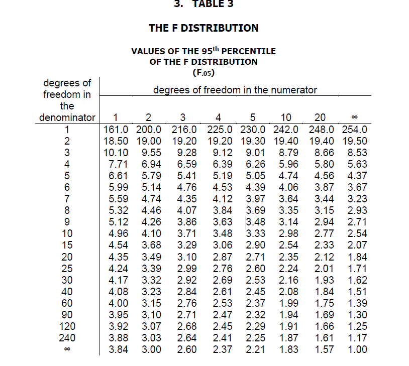
Write down the analysis of variance table for the regression of Y on X1, X2, X3. and X4. Using it and any other information provided above, test for the statistical significance of the overall regression equation and determine which variables should be included and which variables should be deleted (if any). In your answer, state the null hypothesis and alternate hypothesis of all tests performed, compute the test statistics and explain how you arrive at your conclusions (use the attached statistical tables).

For the regression model selected, compute the coefficient of determination and interpret this measure with respect to this application. Be specific in your interpretation.

Obtain a 95% prediction interval for the cost of a 30 second commercial for the prime time comedy program “TWO AND A HALF MEN”. This program has a Nielsen rating of 5.9 and 80% of the audience is in the 18-34 age range.

The non comedy television program, "NCIS", has a rating of 8.2 and 30% of the audience is in the 18-34 age range. The comedy television program "TWO AND A HALF MEN", has a rating of 5.9 and 80% of the audience is in the 18-34 age range. What is the estimated difference in the cost of a 30 second commercial for these two programs (both of these programs are shown during prime time).

Estimate the 25th percentile of the cost of a 30 second commercial for a non comedy prime time program with a Nielsen Rating of 5.0 and with 60% of the audience in the 18-34 age range.

Superbowl 42 was a championship football game played on February 3, 2008 between the New York Giants and the New England Patriots. It received a Nielsen Rating of 43.3. The cost of a 30 second commercial was $2,700,000. This data point was not one of the 45 programs in the sample. Superbowl 42 was a non comedy prime time program with 50% of the audience in the 18-34 age range.

1. Estimate the cost of a 30 second commercial during Superbowl 42, using the appropriate linear regression model.

1. Calculate the residual corresponding to this data point.

1. This data qualifies as an outlier. Explain why.

1. Explain statistically why this model does not work to predict the commercial cost for Superbowl 42. In your answer use only the information that is provided in this problem. Do not use any knowledge that you may have about the game of football. It will not help you answer the question.

QUESTION 2:

In 2008 Superbowl 42 had the second highest Viewership Rating of all time.

Which television program had the highest Viewership rating of all time in 2008? (The Viewership rating represents the number of people who watched the program).

TABLE 1 NORMAL CURVE AREAS

AREAS UNDER THE STANDARD NORMAL CURVE FROM 0 TO Z

Z	0	0.01	0.02	0.03	0.04	0.05	0.06	0.07	0.08	0.09
0.0	0.0000	0.0040	0.0080	0.0120	0.0160	0.0199	0.0239	0.0279	0.0319	0.0359
0.1	0.0398	0.0438	0.0478	0.0517	0.0557	0.0596	0.0636	0.0675	0.0714	0.0753
0.2	0.0793	0.0832	0.0871	0.0910	0.0948	0.0987	0.1026	0.1064	0.1103	0.1141
0.3	0.1179	0.1217	0.1255	0.1293	0.1331	0.1368	0.1406	0.1443	0.1480	0.1517
0.4	0.1554	0.1591	0.1628	0.1664	0.1700	0.1736	0.1772	0.1808	0.1844	0.1879
0.5	0.1915	0.1950	0.1985	0.2019	0.2054	0.2088	0.2123	0.2157	0.2190	0.2224
0.6	0.2257	0.2291	0.2324	0.2357	0.2389	0.2422	0.2454	0.2486	0.2517	0.2549
0.7	0.2580	0.2611	0.2642	0.2673	0.2704	0.2734	0.2764	0.2794	0.2823	0.2852
0.8	0.2881	0.2910	0.2939	0.2967	0.2995	0.3023	0.3051	0.3078	0.3106	0.3133
0.9	0.3159	0.3186	0.3212	0.3238	0.3264	0.3289	0.3315	0.3340	0.3365	0.3389
1.0	0.3413	0.3438	0.3461	0.3485	0.3508	0.3531	0.3554	0.3577	0.3599	0.3621
1.1	0.3643	0.3665	0.3686	0.3708	0.3729	0.3749	0.3770	0.3790	0.3810	0.3830
1.2	0.3849	0.3869	0.3888	0.3907	0.3925	0.3944	0.3962	0.3980	0.3997	0.4015
1.3	0.4032	0.4049	0.4066	0.4082	0.4099	0.4115	0.4131	0.4147	0.4162	0.4177
1.4	0.4192	0.4207	0.4222	0.4236	0.4251	0.4265	0.4279	0.4292	0.4306	0.4319
1.5	0.4332	0.4345	0.4357	0.4370	0.4382	0.4394	0.4406	0.4418	0.4429	0.4441
1.6	0.4452	0.4463	0.4474	0.4484	0.4495	0.4505	0.4515	0.4525	0.4535	0.4545
1.7	0.4554	0.4564	0.4573	0.4582	0.4591	0.4599	0.4608	0.4616	0.4625	0.4633
1.8	0.4641	0.4649	0.4656	0.4664	0.4671	0.4678	0.4686	0.4693	0.4699	0.4706
1.9	0.4713	0.4719	0.4726	0.4732	0.4738	0.4744	0.4750	0.4756	0.4761	0.4767
2.0	0.4772	0.4778	0.4783	0.4788	0.4793	0.4798	0.4803	0.4808	0.4812	0.4817
2.1	0.4821	0.4826	0.4830	0.4834	0.4838	0.4842	0.4846	0.4850	0.4854	0.4857
2.2	0.4861	0.4864	0.4868	0.4871	0.4875	0.4878	0.4881	0.4884	0.4887	0.4890
2.3	0.4893	0.4896	0.4898	0.4901	0.4904	0.4906	0.4909	0.4911	0.4913	0.4916
2.4	0.4918	0.4920	0.4922	0.4925	0.4927	0.4929	0.4931	0.4932	0.4934	0.4936
2.5	0.4938	0.4940	0.4941	0.4943	0.4945	0.4946	0.4948	0.4949	0.4951	0.4952
2.6	0.4953	0.4955	0.4956	0.4957	0.4959	0.4960	0.4961	0.4962	0.4963	0.4964
2.7	0.4965	0.4966	0.4967	0.4968	0.4969	0.4970	0.4971	0.4972	0.4973	0.4974
2.8	0.4974	0.4975	0.4976	0.4977	0.4977	0.4978	0.4979	0.4979	0.4980	0.4981
2.9	0.4981	0.4982	0.4982	0.4983	0.4984	0.4984	0.4985	0.4985	0.4986	0.4986
3.0	0.4987	0.4987	0.4987	0.4988	0.4988	0.4989	0.4989	0.4989	0.4990	0.4990

TABLE 2 THE STUDENT’S T DISTRIBUTION

VALUES OF THE 97.5th PERCENTILE

DEGREES OF FREEDOM.	t.025
1	12.706
2	4.303
3	3.182
4	2.776
5	2.571
6	2.447
7	2.365
8	2.306
9	2.262
10	2.228
11	2.201
12	2.179
13	2.160
14	2.145
15	2.131
16	2.120
17	2.110
18	2.101
19	2.093
20	2.086
21	2.080
22	2.074
23	2.069
24	2.064
25	2.060
26	2.056
27	2.052
28	2.048
29	2.045
infinity	1.960

Please see attached statistics regression problem 1