Week 3 Draft Final PaperFor this assignment, take a moment to review the Final Paper instructions and requirements in Week 6 (included below for reference). You will see that the Final Paper is a disc
Week 3 Instructor Guidance
Week 3 Guidance
MAT 540
Statistical Concepts for Research
One significant component of research involves being able to communicate information visually. This is most often done through tables, graphs, and charts. Last week, you explored various techniques and examples of graphical analysis in research. This week, we begin to outline some ideas for your final paper. In order for a research study to be taken seriously, it must have a clearly outlined and testable hypothesis pertaining to the research question. There are a variety of methods for testing hypotheses, which you will explore in this week’s discussions.
Discrete Probability Distributions
For a discrete variable, simple probability is a ratio of the number of times that a certain event occurs to the number of trials. Probability can be calculated based upon observed trials (experimental probability) or population characteristics (theoretical probability.) Much of statistics is premised on the use of a sample or experiment to draw inferences and conclusions about the un-measurable universal population (theoretical.)
A probability distribution for a discrete variable is a table, which can also be displayed as a bar graph that shows the probability associated with each event for a discrete random variable. For a simple example, consider rolling a single, fair, six-sided die. The outcomes are a roll of 1, 2, 3, 4, 5, or 6, and since the die is fair, each outcome is equally likely. Thus the probability of each outcome is 1/6 (note – this is a theoretical probability.)
We could record this experiment in a probability distribution as:
| Outcome | Probability |
| 1/6 | |
| 1/6 | |
| 1/6 | |
| 1/6 | |
| 1/6 | |
| 1/6 |
Or as a bar graph we get:
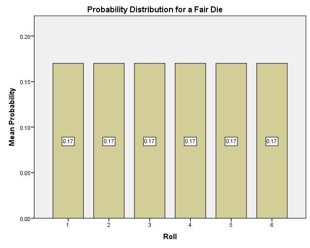
We call this a uniform distribution since every probability is the same and the bars all have a uniform height.
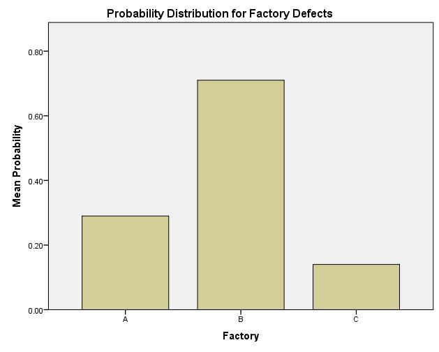
For another example, consider a company with three factories. Factory A has a 2% defect rate, Factory B has a 5% defect rate, and Factory C has a 1% defect rate. If each factory has an equal output, then 1/7th of all defects come from Factory C, 2/7th of all defects come from Factory A, and 5/7th of all defects come from Factory B. We could display the probability distribution as:
Continuous Probability Distribution
As we learned last week, a probability distribution is a graph of the relative frequencies. For a discrete variable, it take the form of a histogram with two properties, that the total area of all the bars is 1 and that the probability of a value between a and b is the sum of the areas of the bars between a and b. If we have a large number of possible values, the histogram looks more and more like a continuous or smooth curve. In Calculus, the idea of the limit is used to answer the question, what happens as the number of possible values goes to infinity. In statistics, we can think if the limit for a discrete variable as a continuous variable. In short, the distribution for a continuous variable is a smooth curve with the following properties:
The total area under the curve is equal to 1, and
The probability of a value between a and b is equal to the area under the curve between a and b.
The curve has all positive values, f(x) >=0 for all x.
These probability density functions can have many different shapes. The have be skewed left, skewed right or symmetric. They can be constant and look like a rectangle (uniform). They can be balanced and symmetric. They can even have sharp cusps.
Some of the descriptive statistics we studied in week one are exhibited in certain characteristics of the distributions. For example, the mode is the highest peak. The median is the vertical line that splits the curve into two equal area pieces. The mean is the balancing point or fulcrum. Variance describes how wide the graph extends.
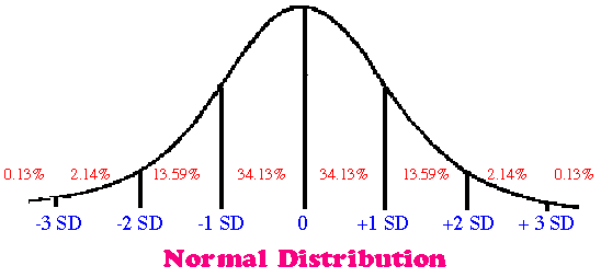
Normal Distribution – The Bell Curve
Watch this
The normal distribution is a specific probability density function in which the mean, median, and mode are all the same. The center of the graph is the highest point and the graph is symmetric. An example is depicted in the header graphic. The normal distribution appears frequently in practice as a limiting value for sample distributions. The exact equation for the normal curve is: ![]()
Where Mu is the mean and sigma is the standard deviation. Often, however, we use the standardized normal curve with a mean of 0 and a standard deviation of 1. The x-values are translated into z-scores by the formula ![]() . Working with one normal curve instead of several allows us to use tables and calculators instead of calculus each time we want to compute areas and thus probabilities.
. Working with one normal curve instead of several allows us to use tables and calculators instead of calculus each time we want to compute areas and thus probabilities.
Distribution of a Sample Mean
Chapter eight describes the basic premise of inferential statistics, sampling from a population. In order to understand whether a sample is representative of the population, we have to understand how the sampling process varies from one sample to another. In this sense, we get into meta-statistics, or statistics about our statistics. The central limit theorem brings it all together and shows that for large n, the distribution of sample means is approximately normal. Thus we can understand and trust our samples by understanding the mean and the variance of our samples. One way we will perform hypothesis testing is by analysis of variance, which is an analysis of how the sample means vary from one to another.
One-Sample Tests
The easiest kind of hypothesis test is one that checks to see if the mean scores of a quantitative variable from a sample matches what is expected for the population (presumed known). Using this kind of a test we can tell if the sample is different enough to be considered statistically significant. In that case, we can make an inference that there is something different about the sample than what was expected. This might be the result of a treatment, sampling bias, or intended effect.
The main steps in hypothesis testing are:
State the Null and Alternative hypothesis
For a one-sample, two-tailed test, this is usually stated as  where # is the presumed known population mean.
Select a Level of Significance
The most common value for alpha for consumer research is 0.05 as a 5% tail is perceived as a reasonable balance between the probability of making a type I and type II error.
Select and Calculate the Test Statistic
Here we determine which kind of a test is appropriate based on the type of variable we have. For a single sample quantitative variable we use a z-test and the z-statistic if the population standard deviation is known. We use a (single-sample) t-test and the t-statistic when the population standard deviation is not known.

Formulate the Decision Rule
In this step we find the critical value(s) for the statistic that separates the general population from the extreme values as determined by the level of significance. Alpha represents the proportion in the tail(s) that are “different enough” to be considered significant.
Make a Rejection Decision
We compare the observed statistic to the critical value(s) to make a rejection decision. If the observed value is inside of the tail (as determined by the critical cut-off values) then we are in the rejection region and we reject the null hypothesis. If the observed statistic is not in the rejection region, then we fail to reject the null hypothesis. Notice that we always make a rejection decision about the Null.
Interpret the Result
Here we contextualize the rejection decision back to the original research question and meaning.
Looking Ahead
Next week, we begin to look at explore how statistical tests can be used to evaluate the evidence provided by the data against the hypothesis. You will review a variety of methods for statistical testing and will also locate an example of statistical testing in research.
Remember to read Chapters 7, 8 and 10. You also have to finish up your draft for the final paper.
Students should be able to do the following:
1. Describe the importance of hypothesis testing.
2. Examine methods of hypothesis testing.
3. Examine the use of statistical tools in research.
Discussions
Participate in the following discussions:
1. Hypothesis Testing 1st Post Due by Day 3. There are strengths and weaknesses
associated with the hypothesis testing procedure. For this discussion, begin by reviewing the concept of hypothesis testing in your textbook and quotes. Based on the quotes, along with this week’s assigned readings and Instructor Guidance, discuss why
hypothesis testing is important in research. Respond to at least two of your classmates’ posts for a minimum grade.
Examples of Hypothesis Testing in Research 1st Post Due by Day 3. Locate an
example of a research study that uses hypothesis testing. Explain whether the study describes its hypothesis testing procedure explicitly or implicitly, based on the explanations in the Methodology section. Finally, discuss what this statistical technique allowed the researchers to accomplish and/or conclude in the study. Respond to at least two of your classmates’ posts for a minimum grade.
Assignments
1. Assignment Homework Problems - Due by Day 6. From Chapter 7, complete Questions 17a, 17b, 17c, 31a, 31b, and 31c. From Chapter 8, complete Questions 33 and 35. From Chapter 10, complete Questions 25 (p-value), 31, 35, and 43. Complete these problems in Connect.
Draft Final Paper- Due by Day 7. For this assignment, take a moment to review the Final Paper instructions and requirements in Week 6. You will see that the Final Paper is a discussion about the use of several statistical techniques used in research studies. While it shares similarities to papers in other classes, you will find that its focus is different. For example, like most assignments, your Final Paper will leverage research studies. However, instead of your analysis focusing on the content of the research study, you will be asked to focus on the statistical tools used in the study and examine how those tools contributed toward the findings in the study. (In other words, the topic of the study itself is irrelevant.) For this Draft Final Paper of two to three double-spaced pages, you will locate three studies, based on the three techniques listed in the Final Paper instructions. Then, address the following items for each of the three research studies you selected:
State the research question being asked.
State which of the three statistical tools the study represents.
Note: There is no need to discuss how the tool is used in the study, as some of the techniques have not yet been covered. No conclusion is needed for this introductory paper.


