In your Week 2 Assignment (attached), you displayed data based on a categorical variable and continuous variable from a specific dataset. In Week 3 (attached), you used the same variables as in Week 2

Running head: INRODUCTION TO QUANTITATIVE ANALYSIS 1

Introduction to Quantitative Analysis: Visually Displaying Data Results

Walden University

Introduction to Quantitative Analysis: Visually Displaying Data Results

According to Wagner (2016), a categorical variable is often nominal or ordinal variable which provides small values of names and labels, while continuous variable that are known as a large values and factions. In reviewing the High School Longitudinal Study dataset, one categorical and one continuous variable will be identified and placed in the appropriate visual display.

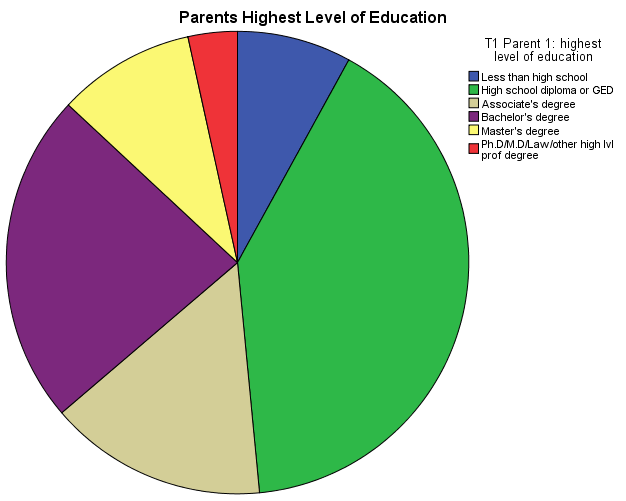
Categorical Variable: Parent Highest Level of Education

For the categorical variable, I will break this down into six categories: less than high school, high school diploma/GED, associate’s degree, bachelor’s degree, master’s degree or decorate.

In your Week 2 Assignment (attached), you displayed data based on a categorical variable and continuous variable from a specific dataset. In Week 3 (attached), you used the same variables as in Week 2 1

Continuous Variable: Years Math Teacher Has Taught High School Math

For the continuous variable, I used the years math teacher has taught high school math. This variable is continuous because it can be broken down into decimals which can be infinite (Wagner, 2016).

Analysis of Data

As I examine the data, both visual allowed to get a holistic view of what’s being presented. For example, the first pie chart identify the level of parent’s education. This allows us to see quick data that majority of parents have a least a high school diploma or GED. However, as I examine Wagner (2016) output data, the data can be analyze by using descriptive functions inside SPSS.

Case Processing Summary
	Cases
Included			Excluded			Total
	Percent			Percent			Percent
T1 Parent 1: highest level of education	16784	71.4%	6719		28.6%	23503		100.0%

Statistics
T1 Parent 1: highest level of education
	Valid	16784
Missing	6719

T1 Parent 1: highest level of education
			Frequency	Percent		Valid Percent	Cumulative Percent
Valid	Less than high school	1342		5.7	8.0		8.0
High school diploma or GED	6795		28.9	40.5		48.5
Associate's degree	2562		10.9	15.3		63.7
Bachelor's degree	3893		16.6	23.2		86.9
Master's degree	1614		6.9	9.6		96.6
Ph.D/M.D/Law/other high lvl prof degree	578		2.5	3.4		100.0
Total	16784		71.4	100.0
Missing	Missing			.0
Unit non-response	6715		28.6
Total	6719		28.6
Total			23503	100.0

Years math teacher has taught high school math
	Valid	17020
Missing	6483

Years math teacher has taught high school math
			Frequency		Percent		Valid Percent	Cumulative Percent
Valid		1288		5.5		7.6		7.6
	1611		6.9		9.5		17.0
	1700		7.2		10.0		27.0
	1260		5.4		7.4		34.4
	1098		4.7		6.5		40.9
	888		3.8		5.2		46.1
	795		3.4		4.7		50.8
	713		3.0		4.2		55.0
	599		2.5		3.5		58.5
10	692		2.9		4.1		62.5
11	547		2.3		3.2		65.8
12	493		2.1		2.9		68.6
13	447		1.9		2.6		71.3
14	438		1.9		2.6		73.8
15	520		2.2		3.1		76.9
16	357		1.5		2.1		79.0
17	275		1.2		1.6		80.6
18	248		1.1		1.5		82.1
19	276		1.2		1.6		83.7
20	356		1.5		2.1		85.8
21	179		.8		1.1		86.8
22	242		1.0		1.4		88.3
23	264		1.1		1.6		89.8
24	144		.6		.8		90.7
25	219		.9		1.3		91.9
26	92		.4		.5		92.5
27	142		.6		.8		93.3
28	141		.6		.8		94.1
29	137		.6		.8		95.0
30	146		.6		.9		95.8
31	713		3.0		4.2		100.0
Total	17020		72.4		100.0
Missing	Missing	50		.2
Unit non-response	6433		27.4
Total	6483		27.6
Total			23503		100.0

In examining this data, this longitudinal study explores teenagers as they process through adulthood. We can clearly identify the different levels of education of parents and determine that a high school diploma were common among them. However, if we look more in depth with the analysis of data, some data is missing which can change the percentage of levels. If we had not ran the report with SPSS, we would never realize that some data were missing, can provide strong possibilities but not 100% accuracy. However, in this sample size, it give us a strong indicator that majority of parents have a least a high school diploma.

As observed in the histogram, most math teachers taught high school math for a least three years, but was it a full three year, or three years and two weeks or months, etc. This analysis of data shows how teachers in their field has years of expertise. However, as we examine both data, one thing to consider is that majority of people will finish high school and it’s important to hire the right teachers to educate these individuals. Therefore, one can say that the importance of a child’s high school experience should be fill with intense knowledge of innovation and solutions in increasing positive social change and community awareness.

Reference:

Wagner, W. E. (2016). Using IBM® SPSS® statistics for research methods and social science statistics (6th ed.). Thousand Oaks, CA: Sage Publications.