the cow jumped
RUNNING HEAD: ONE WAY ANOVA 0
One-Way ANOVA
Stacy Hernandez
PSY7620
Dr. Lorie Fernandez
Capella University
Data Analysis and Application (DAA)
The one way ANOVA is used to determine whether there are any significant differences between the means of two or more independent groups. In this sample, the file grades.sav is used with section (independent variable) and quiz3 (dependent variable).
Data File Description
The one way ANOVA is used to determine whether there are any significant differences between the means of two or more independent groups.
In this sample, the file grades.sav is used with section (independent variable) and quiz3 (dependent variable).
The sample size (N) is 105.
Testing Assumptions
The dependent variable, quiz3, is measured at the interval or ratio level (meaning continuous). The dependent variable (quiz3) in this case, is therefore continuous since it ranges from one to 10. The independent variable (section) should consist of two or more categorical independent groups. In this case, the independent variable (section), has three groups, therefore it meets this assumption. There should be independence of observation, meaning that there is no relationship between the observations in each group or between the groups themselves. There should be no significant outliers, although there are single data points within the data that do not follow a normal pattern. Therefore, the outliers found will a negative effect on the one-way ANOVA, reducing the validity of the results.
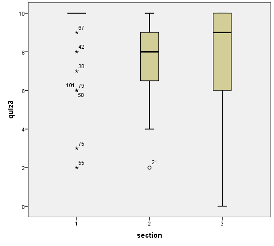
Note the above boxplot indicates outliers in section two, with the id of 21.
The dependent variable (quiz3) should approximately have a normal distribution for each category of the independent variable (section). The null hypothesis is that the data is of a normal distribution, that the mean (average value of the dependent variable) is the same for all groups.
Ho – the observed distribution fits the normal distribution.
The alternative hypothesis is that the data does not have a normal distribution; the average is not the same for all groups.
Ha – the observed distribution does not fit the normal distribution.
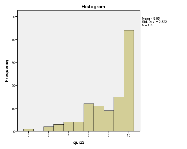
It is observed that the data is not normally distributed. Most sections have quiz3 values between five and nine note this is a visual estimate. Note that the largest group also has the largest value of quiz3. The statistics from the histogram of quiz3 reveal that the Mean is 8.05; the Standard Deviation is 2.322, with a total number N of 105.
| Descriptive Statistics | ||||||||||
| N | Minimum | Maximum | Mean | Std. Deviation | Skewness | Kurtosis | ||||
| Statistic | Statistic | Statistic | Statistic | Statistic | Statistic | Std. Error | Statistic | Std. Error | ||
| quiz3 | 105 | 0 | 10 | 8.05 | 2.322 | -1.177 | .236 | .805 | .467 | |
| section | 105 | 1 | 3 | 2.00 | .797 | .000 | .236 | -1.419 | .467 | |
| Valid N | 105 | |||||||||
When looking at skewness, for a perfectly normal and symmetrical distribution, it has a value of zero (Warner, 2013). There tends to be a quantification of how symmetrical the distribution is (Warner, 2013). In this sample, the skewness is -1.177. This presents an indication of an asymmetrical distribution with a long tail to the left, or a Left Skewed Distribution. The Kurtosis is an indicator used in distribution analysis to see if there is a sign of a flatter (Platykurtic) than an ideal normal distribution (Warner, 2013). If the distribution has a sharper or steeper peak in the center than an ideal distribution, it is considered leptokurtic (Warner, 2013). The kurtosis here is .805 (a normal distribution corresponds to a value of 3); hence indicating that it is a Platykurtic distribution.
| Tests of Normality | ||||||||
| section | Kolmogorov-Smirnova | Shapiro-Wilk | ||||||
| Statistic | df | Sig. | Statistic | df | Sig. | |||
| quiz3 | .440 | 33 | .000 | .550 | 33 | .000 | ||
| .156 | 39 | .018 | .909 | 39 | .004 | |||
| .223 | 33 | .000 | .853 | 33 | .000 | |||
| a. Lilliefors Significance Correction | ||||||||
Considering that the data is smaller than 2000 elements, using the Shapiro-Wilk test is best. The p-value is 0.000 for section one; therefore the null hypothesis will be rejected. The p-value is 0.004 for section two, hence the rejection of the null hypothesis. The p-value for section three is 0.000; the null hypothesis will also be rejected. The reason for the rejection of the null hypotheses is that the data is not normally distributed for all the groups
| Test of Homogeneity of Variances | |||
| quiz3 | |||
| Levene Statistic | df1 | df2 | Sig. |
| 1.576 | 2 | 102 | .212 |
The homogeneity of variances refers to the assumption that the variances of populations being compared are equal (using ANOVA). They can be tested by using the Levene test (Warner, 2013). There is a need for homogeneity of variances, the Levene tests for the null assumption that the population variances are equal (Warner, 2013).
Ho – Population variances are equal
Ha – Population variances are not equal
In the above Levene statistic, it shows a sig value of .212, which is clearly above .05, the preselected alpha level, therefore the decision, is not to reject the Ho. This clearly shows that the homogeneity was not violated.
It is clear that most of the assumptions of the one-way ANOVA have been met. The dependent variable, quiz3, has a range of one through 10, so therefore it is continuous. The independent variable, section, has three categorized groups. These groups do not have a relationship between the categorical groups. The assumption of a lack of outliers in section 2 has not been fully met. There is an existence of outliers in section two as represented by circles and in section 1 represented by stars.
Analyzing the Levene test there was the discovery that there is homogeneity of variances. Although the assumption of normality of data has not been met by the three groups, no surprise due to real world data being used. Over all it is concluded that the assumptions are met.
Research Question
Will there be a significant difference between the sections of the quiz given?
Hypotheses
Null Hypothesis – There is no difference in quiz3 by the sections.
Alternative Hypothesis – There is a difference in quiz the by section.
Alpha Level
Alpha level is 0.05
Interpretation
Means Plot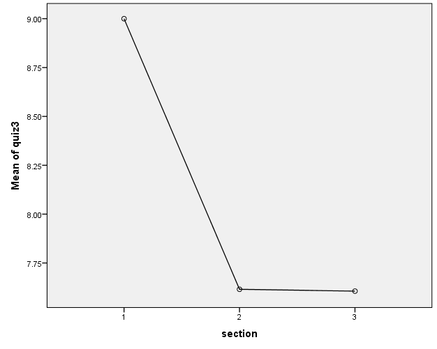
The ANOVA means plot will provide a visual representation of the group means and their linear relationship (Warren, 2013). The mean score on quiz3 of section 1 (9.00) is appeared to be significantly different from those of section 2 (7.62) and section 3 (7.61) when we observe the descriptive statistics and the mean plot. The results of ANOVA indicated that the differences among the means scores on quiz3 for the 3 sections were only due to chance causes, actually there is no effect of the section in which the student is studying on the score, F (2, 102) = 3.058, p = 0.051 > 0.05.
| Case Processing Summary | ||||||
| Cases | ||||||
| Included | Excluded | Total | ||||
| N | Percent | N | Percent | N | Percent | |
| quiz3 * section | 105 | 100.0% | 0 | 0.0% | 105 | 100.0% |
| Report | |||
| quiz3 | |||
| Section | Mean | N | Std. Deviation |
| 9.00 | 33 | 2.107 | |
| 7.62 | 39 | 2.098 | |
| 7.61 | 33 | 2.549 | |
| Total | 8.05 | 105 | 2.322 |
| ANOVA | |||||
| quiz3 | |||||
| Sum of Squares | df | Mean Square | F | Sig. | |
| Between Groups | 43.652 | 2 | 21.826 | 4.305 | .016 |
| Within Groups | 517.110 | 102 | 5.070 | ||
| Total | 560.762 | 104 | |||
Degrees of Freedom
There are two degrees of freedom between the group’s estimate of variance, and 102 degrees of freedom within the group’s variance.
F Value
The F value is 4.305
P Value
The p value is 0.016. This is less than the α level therefore we reject Ho.
Calculated Effect Size
The effect size is the size of an effect; it is shown that there is a significant difference between groups. The difference in means between:
1 and 2 is 1.385
1 and 3 is 1.394
2 and 1 is -1.385
2 and 3 is 0.009
3 and 1 is -1.394
3 and 2 is -0.009
This is shown in the Post-Hoc Tet below.
| Multiple Comparisons | ||||||
| Dependent Variable: quiz3 | ||||||
| Tukey HSD | ||||||
| (I) section | (J) section | Mean Difference (I-J) | Std. Error | Sig. | 95% Confidence Interval | |
| Lower Bound | Upper Bound | |||||
| 1.385* | .533 | .029 | .12 | 2.65 | ||
| 1.394* | .554 | .036 | .08 | 2.71 | ||
| -1.385* | .533 | .029 | -2.65 | -.12 | ||
| .009 | .533 | 1.000 | -1.26 | 1.28 | ||
| -1.394* | .554 | .036 | -2.71 | -.08 | ||
| -.009 | .533 | 1.000 | -1.28 | 1.26 | ||
| *. The mean difference is significant at the 0.05 level. | ||||||
Post-Hoc Test
If the significance is less than the alpha level of 0.05, there would be a need to reject the null hypothesis. Therefore, in all the cases with the exception of two the null hypothesis will be rejected.
Conclusion
After performing the one-way ANOVA, the significance was less than the alpha level. Hence, it is valid to say that the null hypothesis is rejected.
Strengths
The one-way ANOVA can be used to compare data for more than two groups. It has the ability to have control over Type I errors. The one-way ANOVA also displays a robust design, which increases statistical power because it is a parametric test. It provides the overall test of equality of group of means.
Limitations
Just as the one-way ANOVA has it strengths, it also had its weaknesses, or limitations. The greatest one would be that it does require a population distribution that is normal. If the null hypothesis is rejected, it means at least one group differs from the others, but with the one-way ANOVA, and multiple groups, and can become difficult to determine which group is different. The test also assumes equality of variances, and all assumptions need to be fulfilled.
References
Warner, R. M. (2013). Applied statistics from bivariate through multivariate techniques (2nd ed.). Thousand Oaks, California, United States: Sage Publications.


