2-3 paragraph SPSS
Week 2 Assignment: Visual display of data
For week 2 assignment on visual display of data, I have used the Afrobarometer dataset. I have chosen one categorical and one continuous variable as required. A variable is said to be categorical if it can take distinct values (Frankfort, et al. 2015), for example yes or no. From this definition, I have chosen gender of the respondent as my categorical variable for this analysis.
Similarly, a variable is said to be continuous if it can take a range of values or uncountable number values in given range of values (Frankfort, et al. 2015). An example of a continuous variable is the weight of a person. which can take infinite values including fractions and whole numbers. From the forgoing illustration, I have decided to choose age as my continuous variable. This is because age can take infinitely many values both fraction and whole numbers.
For the visual display of data, I have chosen a bar chart to analyse the continuous variable-the age of the respondents. The age category variable can be best described using the bar chart.
The output of the SPSS analysis is shown in figure 1 below. Lengths of the bars represents the number of respondents in each category of age bracket. The y-axis represents the frequency (the number) of respondents while the x-axis represents the different age brackets. From the graph, we can clearly see that the age bracket with the highest number of respondents is 18-35, followed by 36-50 and the bracket with the lowest number of respondents 51 years and above. This indicates that majority of the respondents are in the age bracket of the working group and few have reached their retirement age.
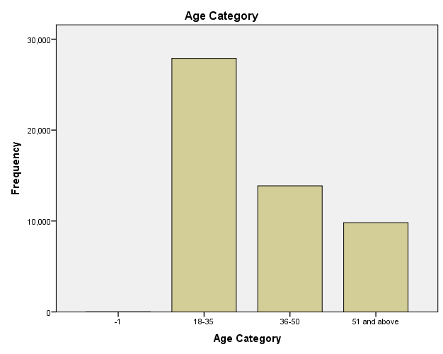
Figure1
For the analysis of categorical data, I have chosen to use the frequency table. My major interest to compare the representation by proportion of both the male and the female respondents.
From output is in table 1 below and we can clearly see that there were many female respondents (25817) than their counterpart male respondents (25770). The difference between the male and female respondents (47) was statistically large/significance, since it is more than 30. Looking at the percentage however, both the male and the female respondents had 50% representation. From this, we can say that the sample was gender sensitive and this is very important since it minimises the elements of biasedness towards a give gender. We can also see from the table that the total number of respondents was 51587. This is significant since it tells us the sample size of the study. Lastly, we can see from the table that all the entries were valid. This is also significant since it minimises the cases of sampling error.
| Q101. Gender of respondent | |||||
| Frequency | Percent | Valid Percent | Cumulative Percent | ||
| Valid | Male | 25770 | 50.0 | 50.0 | 50.0 |
| Female | 25817 | 50.0 | 50.0 | 100.0 | |
| Total | 51587 | 100.0 | 100.0 | ||
Table 1
References
Frankfort-Nachias, C., & Leon-Guerrero, A. (2015). Social Statistics for a diverse society,
(7thed.). Thousand Oaks, CA: Sage Publications.
Walden University writing centre. (n.d). General guidance on data display.


