VibrationQuestions-NII

class: Vibrations

Guidelines:

• For Each problem start with a Free Body Diagram (FBD) first then start solving each point.

• when you solve it please Do it NEATLY organized perfectly, so when i submit it, i just print it and thats it.

- You must satisfy all the requirements in details. for example, when it asks you to use a specific command, please do it. do not solve any problem in other functions even if it gives you the same answer.

1. Periodic Forcing Function of a SDOF system (base excitation).

m = 20kg, c = 100Ns/m, k = 500N/m, Y = 0.5m, w = 1Hz

1. 1. Write out the equation of motion with available values.

   2. Using the ss command in Matlab, define a LTI system that represents the base excitation problem shown above.

   3. Define the base displacement equation in Matlab.

   4. Simulate the response of the system to the base excitation using the lsim command (note: that is l as in linear, not the number one) for at least 10 sec.

   5. Find the Fourier coefficients of the forcing function show above. You can use the fft command in Matlab.

   6. Approximate the forcing function using the first 5 Fourier coefficients (j =0 to 5) and simulate the response of the system to this approximated forcing function.

   7. Approximate the forcing function using the first 15 Fourier coefficients (j =0 to 5) and simulate the response of the system to this approximated forcing function.

   8. Plot the responses of the system to the original forcing function from part d, and the approximated forcing functions in parts f and g. Properly label all figures.

1. Non-Periodic Forcing Function of a SDOF system.

A mass-spring-damper is externally forced with m = 10kg, c = 200Ns/m, k = 500N/m and the forcing function is below.

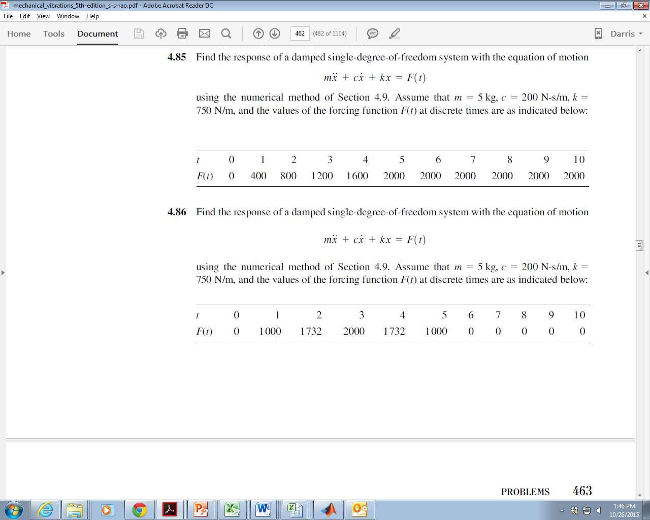
1. 1. Write out the equation of motion with available values.

   2. Using the ss command in Matlab, define a LTI system that represents the externally forced problem.

   3. Define the forcing function in Matlab as an array.

   4. Simulate the response of the system to the excitation force using the lsim command (note: that is l as in linear, not the number one) for at least 10 sec.

   5. Define the forcing function in Matlab as a ½ sine function with amplitude 2000 but sample the function at 100 Hz. The function should go from 0 to 10 but now have 1001 data points instead of 11.

   6. Simulate the response of the system to the resampled excitation force using the lsim command (note: that is l as in linear, not the number one).

   7. Plot both results and compare. Properly label all figures.

1. Multiple Degree of Freedom – Harmonic Forcing.

A heavy machine tool is mounted on a suspended floor. The machine, the machine base and the floor can be modeled as a three degree of freedom system.

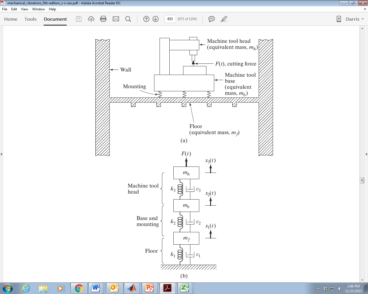
1. 1. Derive the equations of motion and write them out in matrix form

   2. Using the ss command in Matlab, define a LTI system. Starting with part b, you can use the following values for this problem k1 = 5000 lb/in, k2 = 2000 lb/in, k3 = 2000 lb/in, c1 = 10 lb-sec/in, c2 = 20 lb-sec/in, c3 = 5, mf = 500 slugs, mb = 100 slugs, and mh = 10 slugs.

   3. What are the natural frequencies of this system using the eig command?

   4. What are the normalized mode shapes of this system (show all three and associate them with their respective natural frequency)?

   5. If the machining process results in a forcing function of 1000 cos (60t), acting on mass mh, find the steady state response of the system. Plot x1, x2 and x3 on separate, properly labeled graphs. Run the simulation for a sufficient time that the homogenous (transient) response has dissipated.

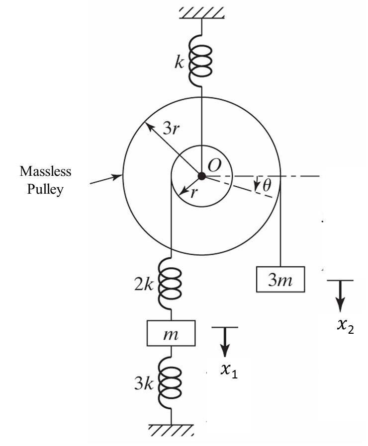
1. 2-DOF Vibration

A massless pulley connects two masses together. k = 1000 N/m and m = 20 kg

1. 1. Write the Equations of Motion in Matrix Form

   2. Find the natural frequencies

   3. Find the mode shapes

   4. Use the ss command in Matlab to create an LTI model of this system.

   5. Plot the response of the system (X1 and X2) when an initial displacement of 0.1m is applied to X1.

   6. Apply a unit sine wave at X1 with a frequency of excitation that is ½ of the lowest natural frequency and plot the response. Include the displacement of both degrees of freedom on the same plot and label appropriately.

   7. Apply a unit sine wave at X1 with a frequency of excitation that is twice of the highest natural frequency and plot the response. Include the displacement of both degrees of freedom on the same plot and label appropriately.

1. 2-DOF Free Vibration

A rigid rod of negligible mass and length 2L is pivoted at the middle point and is constrained to move in the vertical plane by springs and masses, as shown. L = 1ft, m = 10 slugs, k = 100 lb/in

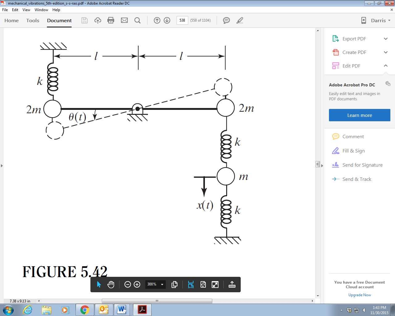
1. 1. Write the Equations of Motion in Matrix Form

   2. Find the natural frequencies

   3. Find the mode shapes

   4. Use the ss command in Matlab to create an LTI model of this system.

   5. Plot the response of the system (X and Ɵ) when an initial displacement of 0.1m is applied to X.

   6. Apply a unit sine wave at X with a frequency of excitation that is ½ of the lowest natural frequency and plot the response. Include the displacement of both degrees of freedom on the same plot and label appropriately.

   7. Apply a unit sine wave at X with a frequency of excitation that is twice of the highest natural frequency and plot the response. Include the displacement of both degrees of freedom on the same plot and label appropriately.