Urgent SPSS Case Analysis-Needs Fixing
![]()
The variable used in the analysis is “Friendly Employees”. An independent sample t-test is conducted to compare, “friendly employees,” between Jose’s South-western Café(M=4.80,SD=0.489) and Santa Fe Grill(M=2.94,S.D=0.947).The result showed significant difference in the ,”Friendly Employee” between Jose Southwestern Café and Santa Fe Grill with t-value of t(395.25) =26.025 with the p-value being 0.000.
| Group Statistics | |||||
| Favorite Mexican Restaurant | N | Mean | Std. Deviation | Std. Error Mean | |
| X12 -- Friendly Employees | Jose's Southwestern Cafe | 152 | 4.80 | .489 | .040 |
| Santa Fe Grill | 253 | 2.94 | .947 | .060 | |
| Independent Samples Test | |||||||||||||||||||
| Levene's Test for Equality of Variances | t-test for Equality of Means | ||||||||||||||||||
| F | Sig. | t | df | Sig. (2-tailed) | Mean Difference | Std. Error Difference | 95% Confidence Interval of the Difference | ||||||||||||
| Lower | Upper | ||||||||||||||||||
| X12 -- Friendly Employees | Equal variances assumed | 178.737 | .000 | 22.494 | 403 | .000 | 1.862 | .083 | 1.699 | 2.025 | |||||||||
| Equal variances not assumed | 26.025 | 395.295 | .000 | 1.862 | .072 | 1.721 | 2.003 | ||||||||||||

Answer
The variable used in the analysis is “Satisfaction”. An independent sample t-test is conducted to compare, “Satisfaction,” between Jose’s South-western Café(M=5.31,SD=1.141) and Santa Fe Grill(M=4.54,S.D=1.002).The result showed significant difference in the ,”Satisfaction” between Jose Southwestern Café and Santa Fe Grill with t-value of t(286.47) =6.86 with the p-value being 0.000.
| Group Statistics | |||||
| Favorite Mexican Restaurant | N | Mean | Std. Deviation | Std. Error Mean | |
| X22 -- Satisfaction | Jose's Southwestern Cafe | 152 | 5.31 | 1.141 | .093 |
| Santa Fe Grill | 253 | 4.54 | 1.002 | .063 | |
| Independent Samples Test | ||||||||||||||||||||
| Levene's Test for Equality of Variances | t-test for Equality of Means | |||||||||||||||||||
| F | Sig. | t | df | Sig. (2-tailed) | Mean Difference | Std. Error Difference | 95% Confidence Interval of the Difference | |||||||||||||
| Lower | Upper | |||||||||||||||||||
| X22 -- Satisfaction | Equal variances assumed | 3.957 | .047 | 7.085 | 403 | .000 | .768 | .108 | .555 | .981 | ||||||||||
| Equal variances not assumed | 6.860 | 286.468 | .000 | .768 | .112 | .547 | .988 | |||||||||||||
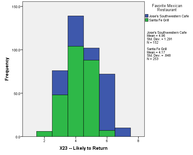
The variable is the,” Likely to return”. The likelihood of returning to Santa Fe Grill and Jose’s Southwestern Café was found out using cross-tab in SPSS. The result showed 0% are highly likely to return to Santa Fe Grill whereas 6.6% are highly likely to return to Jose’s Southwestern Café. It is further evident from the stacked bar graph as shown below. The mean value for Jose’s Southwestern café,” likely to return” obtained was 4.96 with SD =1.291, whereas for Jose’s South Western café, “likely to return” was 4.17 with SD =0.848.
| Case Processing Summary | ||||||
| Cases | ||||||
| Valid | Missing | Total | ||||
| N | Percent | N | Percent | N | Percent | |
| Favorite Mexican Restaurant * X23 -- Likely to Return | 405 | 100.0% | 0 | 0.0% | 405 | 100.0% |
| Favorite Mexican Restaurant * X23 -- Likely to Return Cross tabulation | |||||||||||||||||
| X23 -- Likely to Return | Total | ||||||||||||||||
| 2 | 3 | 4 | 5 | 6 | Highly Likely | ||||||||||||
| Favorite Mexican Restaurant | Jose's Southwestern Cafe | Count | 0 | 28 | 35 | 14 | 65 | 10 | 152 | ||||||||
| % within Favorite Mexican Restaurant | 0.0% | 18.4% | 23.0% | 9.2% | 42.8% | 6.6% | 100.0% | ||||||||||
| Santa Fe Grill | Count | 6 | 48 | 104 | 88 | 7 | 0 | 253 | |||||||||
| % within Favorite Mexican Restaurant | 2.4% | 19.0% | 41.1% | 34.8% | 2.8% | 0.0% | 100.0% | ||||||||||
| Total | Count | 6 | 76 | 139 | 102 | 72 | 10 | 405 | |||||||||
| % within Favorite Mexican Restaurant | 1.5% | 18.8% | 34.3% | 25.2% | 17.8% | 2.5% | 100.0% | ||||||||||

The variable used are as follows:
Try New and Different Thing-X1
Buy New Products-X9
Try New Brands-X11
The descriptive statistics table shows man value of X1 being 5.39 with SD=1.863.The mean value of X9= 5.60 with SD= 1.606 and mean of X11 = 5.42 with SD =1.766.
A bivariate correlation test was used to compare the relationship among items X1,X9 and X11.The result showed the correlation between r(X1,X9)= 0.688,p= 0.000.Thus,positive significant correlation exists between X1 and X9.
The correlation coefficient between X1 and X11,r(X1,X11)=0.844,p-value =0.000.A positive and significant correlation exists between X1 and X11.
The correlation coefficient between X9 and X11,r(X9,X11)=0.693,p-value =0.000.A positive and significant correlation exists between X9 and X11.
Here positive correlation means increase in value of one of the variable causes an increase in another variable.
| Report | |||
| X1 -- Try New and Different Things | X9 -- Buy New Products | X11 -- Try New Brands | |
| Mean | 5.39 | 5.60 | 5.42 |
| 405 | 405 | 405 | |
| Std. Deviation | 1.863 | 1.606 | 1.766 |
| Correlations | |||||||
| X1 -- Try New and Different Things | X9 -- Buy New Products | X11 -- Try New Brands | |||||
| X1 -- Try New and Different Things | Pearson Correlation | 1 | .688** | .844** | |||
| Sig. (2-tailed) | .000 | .000 | |||||
| 405 | 405 | 405 | |||||
| X9 -- Buy New Products | Pearson Correlation | .688** | 1 | .693** | |||
| Sig. (2-tailed) | .000 | .000 | |||||
| 405 | 405 | 405 | |||||
| X11 -- Try New Brands | Pearson Correlation | .844** | .693** | 1 | |||
| Sig. (2-tailed) | .000 | .000 | |||||
| 405 | 405 | 405 | |||||
| **. Correlation is significant at the 0.01 level (2-tailed). | |||||||

Answer
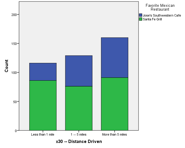
The variable is ,”Distance Driven”.which is ordinal.Therefore the appropriate test will be the Mann Whitney U test which is the non-parametric version of independent sample t-test.
The mean rank for distance driven for Jose’s South-western Café is 222.42 whereas the mean rank for Santa Fe Grill obtained is 191.33.The second table showed test statistic value of U=16276.5 with the p-value of 0.006.Further,it was analysed through stacked bar graph which showed large difference in each categories
| Ranks | ||||
| Favorite Mexican Restaurant | N | Mean Rank | Sum of Ranks | |
| x30 -- Distance Driven | Jose's Southwestern Cafe | 152 | 222.42 | 33807.50 |
| Santa Fe Grill | 253 | 191.33 | 48407.50 | |
| Total | 405 | |||
| Test Statisticsa | |
| x30 -- Distance Driven | |
| Mann-Whitney U | 16276.500 |
| Wilcoxon W | 48407.500 |
| -2.754 | |
| Asymp. Sig. (2-tailed) | .006 |
| a. Grouping Variable: Favorite Mexican Restaurant | |
Stacked Bar graph

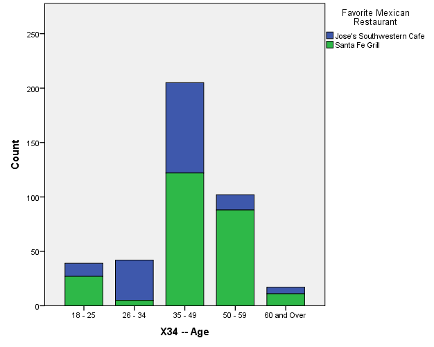
The variable is ,”Distance Driven”.which is ordinal.Therefore the appropriate test will be the Mann Whitney U test which is the non-parametric version of independent sample t-test.
The mean rank for distance driven for Jose’s South-western Café is 222.42 whereas the mean rank for Santa Fe Grill obtained is 191.33.The second table showed test statistic value of U=16276.5 with the p-value of 0.006.Further,it was analysed through stacked bar graph which showed large difference in each categories
| Ranks | ||||
| Favorite Mexican Restaurant | N | Mean Rank | Sum of Ranks | |
| X34 -- Age | Jose's Southwestern Cafe | 152 | 163.54 | 24857.50 |
| Santa Fe Grill | 253 | 226.71 | 57357.50 | |
| Total | 405 | |||
| Test Statisticsa | |
| X34 -- Age | |
| Mann-Whitney U | 13229.500 |
| Wilcoxon W | 24857.500 |
| -5.696 | |
| Asymp. Sig. (2-tailed) | .000 |
| a. Grouping Variable: Favorite Mexican Restaurant | |
Answer
The variable Healthy_Food was computed by adding the following variable:
X4-Avoid Fried Foods
X8-Eat balanced Nutritious Meals
X10-Careful about what I eat
The mean value for Jose’s Southwestern Café obtained was 10.73 with SD =2.23 whereas the mean value of Santa Fe Grill obtained was 14.54 with SD =3. 002.An independent sample t-test was used to compare the mean difference between Jose’s Southwestern Café and Santa Fe Grill with respect to Healthy Food. The result showed test statistic value of t (385) = -14.56 with the p-value of 0. 000.Thus the difference is significant between Jose’s Southwestern Café and Santa Fe Grill with respect to Healthy_Food.
| Group Statistics | |||||
| Favorite Mexican Restaurant | N | Mean | Std. Deviation | Std. Error Mean | |
| Healthy_Food | Jose's Southwestern Cafe | 152 | 10.7303 | 2.23153 | .18100 |
| Santa Fe Grill | 253 | 14.5375 | 3.00191 | .18873 | |
| Independent Samples Test | |||||||||||
| Levene's Test for Equality of Variances | t-test for Equality of Means | ||||||||||
| F | Sig. | t | df | Sig. (2-tailed) | Mean Difference | Std. Error Difference | 95% Confidence Interval of the Difference | ||||
| Lower | Upper | ||||||||||
| Healthy_Food | Equal variances assumed | 19.707 | .000 | -13.546 | 403 | .000 | -3.80729 | .28106 | -4.35981 | -3.25476 | |
| Equal variances not assumed | -14.560 | 385.080 | .000 | -3.80729 | .26150 | -4.32142 | -3.29315 | ||||
Answer
The regression model for Santa Fe customers was developed considering the following variables:
Dependent Variable:X22-Satisfaction
Independent Variable:X12-Friendly Employees, X14-Large Size Portions, X15-Fresh Food.
The first table shows coefficient of determination being R-square = 0.629 meaning 62.9% of the variation in satisfaction is explained by variable, X12(friendly employees), X14(Large Size Portions) and X15(Fresh Food).
The second table shows whether the overall regression model is significant or not. The result shows F-value of F (3,249) =141.017 with the p-value of 0.000 meaning the overall regression is significant.
The third table is the individual independent variable interpretation.
The model can be represented as
 ----------------------- (1)
From the above model it is clear increase in 1 unit of friendly employees cause an increase of 0.436 unit of satisfaction. The test statistic obtained is t =9.999 with p-value =0.000.
The equation (1) shows that unit increase of,” Large Size Portions” cause an increase of 0.123 increase of satisfaction. The test statistic obtained is t =4.293 with p-value =0.000, meaning the slope is significant.
The equation (1) shows that unit increase of,” Fresh food” cause an increase of 0.559 increase of satisfaction. The test statistic obtained is t =15.403 with p-value =0.000, meaning the slope is significant.
The most important variable would be the variable that brings the most satisfaction per unit increase in independent variable. It can be obtained from the standardized coefficient of the regression(beta). Thus from the above regression model it is clear that the most important variable is,” Fresh food-X15(beta=0.649)” and the least important variable is.” Large Portion-X14(beta=0.182)”.
| Model Summary | ||||
| Model | R | R Square | Adjusted R Square | Std. Error of the Estimate |
| .793a | .629 | .625 | .613 | |
| a. Predictors: (Constant), X15 -- Fresh Food, X12 -- Friendly Employees, X14 -- Large Size Portions | ||||
| ANOVAa | ||||||
| Model | Sum of Squares | df | Mean Square | F | Sig. | |
| Regression | 159.145 | 3 | 53.048 | 141.017 | .000b | |
| Residual | 93.670 | 249 | .376 | |||
| Total | 252.814 | 252 | ||||
| a. Dependent Variable: X22 -- Satisfaction | ||||||
| b. Predictors: (Constant), X15 -- Fresh Food, X12 -- Friendly Employees, X14 -- Large Size Portions | ||||||
| | ||||||
| | ||||||
| Coefficients | ||||||
| Model | Unstandardized Coefficients | Standardized Coefficients | t | Sig. | ||
| B | Std. Error | Beta | ||||
| (Constant) | -.242 | .238 | -1.016 | .311 | ||
| X12 -- Friendly Employees | .436 | .044 | .412 | 9.999 | .000 | |
| X14 -- Large Size Portions | .123 | .029 | .182 | 4.293 | .000 | |
| X15 -- Fresh Food | .559 | .036 | .649 | 15.403 | .000 | |
| a. Dependent Variable: X22 -- Satisfaction | ||||||


