Statistics assignment

EXERCISE 10

Description of a Study Sample

STATISTICAL TECHNIQUE IN REVIEW

Most research reports describe the subjects or participants who comprise the study sample. This description of the sample is called the sample characteristics, which may be presented in a table and/or the narrative of the article. The sample characteristics are often presented for each of the groups in a study (i.e., intervention and control groups). Descriptive statistics are calculated to generate sample characteristics, and the type of statistic conducted depends on the level of measurement of the demographic variables included in a study (Grove, Burns, & Gray, 2013 ). For example, data collected on gender is nominal level and can be described using frequencies, percentages, and mode. Measuring educational level usually produces ordinal data that can be described using frequencies, percentages, mode, median, and range. Obtaining each subject’ s specific age is an example of ratio data that can be described using mean, range, and standard deviation. Interval and ratio data are analyzed with the same statistical techniques and are some-times referred to as interval/ratio-level data in this text.

RESEARCH ARTICLE

Source Oh, E. G., Yoo, J. Y., Lee, J. E., Hyun, S. S., Ko, I. S., & Chu, S. H. (2014). Effects of a three-month therapeutic lifestyle modification program to improve bone health in postmenopausal Korean women in a rural community: A randomized controlled trial. Research in Nursing & Health, 37 (4), 292–301.

Introduction

Oh and colleagues (2014) conducted a randomized controlled trial (RCT) to examine the effects of a therapeutic lifestyle modification (TLM) intervention on the knowledge, self-efficacy, and behaviors related to bone health in postmenopausal women in a rural com-munity. The study was conducted using a pretest-posttest control group design with a sample of 41 women randomly assigned to either the intervention n = 21) or control group ( n = 20). “The intervention group completed a 12-week, 24-session TLM program of individualized health monitoring, group health education, exercise, and calcium–vitamin D supplementation. Compared with the control group, the intervention group showed significant increases in knowledge and self-efficacy and improvement in diet and exercise after 12 weeks, providing evidence that a comprehensive TLM program can be effective in improving health behaviors to maintain bone health in women at high risk of osteoporosis” (Oh et al., 2014 p. 292).

Relevant Study Results

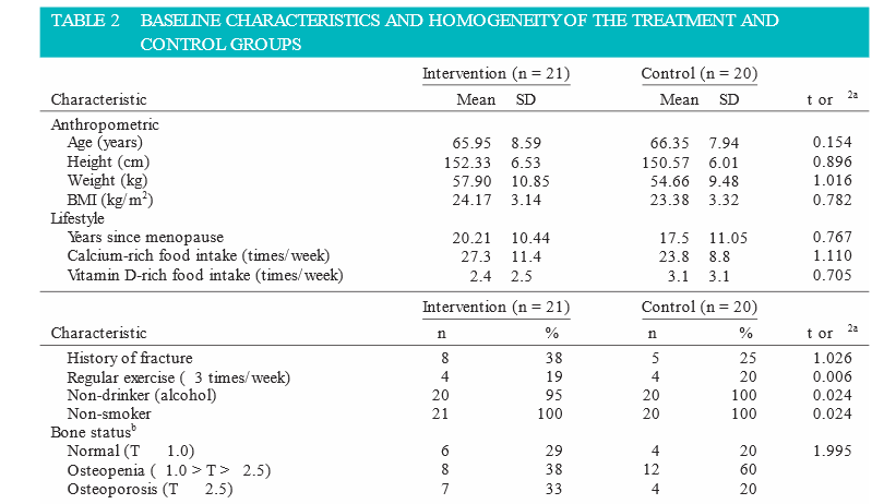
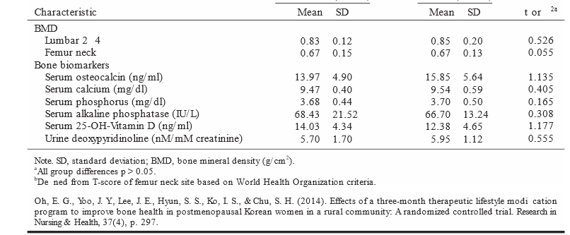
“Bone mineral density (BMD; g/cm 2) was measured by dual energy x-ray absorptiometry (DXA) with the use of a DEXXUM T machine. A daily calibration inspection was per-formed. The error rate for these scans is less than 1%. Based on the BMD data, the participants were classified into three groups: osteoporosis (a BMD T -score less than − 2.5); osteopenia (a BMD T -score between − 2.5 and − 1.0); and normal bone density (a BMD T -score higher than − 1.0)” (Oh et al. 2014 , p. 295). “

Characteristics of Participants

The study participants were 51–83 years old, and the mean age was 66.2 years (SD = 8.2). The mean BMI was 23.8 kg/m 2 (SD = 3.2). Most participants did not consume alcoholic drinks, and all were nonsmokers. Antihypertensive and analgesics such as aspirin and acetaminophen were the most common medications taken by the participants. Less than 20% of participants had a regular routine of exercise at least three times per week. Daily calcium- and vitamin D-rich food intake (e.g., dairy products, fish oil, meat, and eggs) was low. Seventy-five percent ( n = 31) of the participants had osteoporosis or osteopenia. There were no differences in the baseline characteristics of the groups (Table 2 ). The adherence rate to the TLM program was 99.6%” (Oh et al., 2014, p. 296).

QUESTIONS.

1. What demographic variables were measured at the nominal level of measurement in the Oh et al. (2014) study? Provide a rationale for your answer.

2. What statistics were calculated to describe body mass index (BMI) in this study? Were these appropriate? Provide a rationale for your answer.

3. Were the distributions of scores for BMI similar for the intervention and control groups? Provide a rationale for your answer.

4. Was there a significant difference in BMI between the intervention and control groups? Provide a rationale for your answer.

5. Based on the sample size of N = 41, what frequency and percentage of the sample smoked? What frequency and percentage of the sample were non-drinkers (alcohol)? Show your calculations and round to the nearest whole percent.

6. What measurement method was used to measure the bone mineral density (BMD) for the study participants? Discuss the quality of this measurement method and document your response.

7. What statistic was calculated to determine differences between the intervention and control groups for the lumbar and femur neck BMDs? Were the groups significantly different for BMDs?

8. The researchers stated that there were no significant differences in the baseline characteristics of the intervention and control groups (see Table 2). Are these groups heterogeneous or homo-generous at the beginning of the study? Why is this important in testing the effectiveness of the therapeutic lifestyle modification (TLM) program?

9. Oh et al. (2014, p. 296) stated that “the adherence rate to the TLM program was 99.6%.” Discuss the importance of intervention adherence, and document your response.

10. Was the sample for this study adequately described? Provide a rationale for your answer.

EXERCISE 26

Determining the Normality of a Distribution

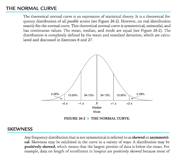
Most parametric statistics require that the variables being studied are normally distributed. The normal curve has a symmetrical or equal distribution of scores around the mean with a small number of outliers in the two tails. The first step to determining normality is to create a frequency distribution of the variable(s) being studied. A frequency distribution can be displayed in a table or figure. A line graph figure can be created whereby the x axis consists of the possible values of that variable, and the y axis is the tally of each value. The frequency distributions presented in this Exercise focus on values of continuous variables. With a continuous variable, higher numbers represent more of that variable and the lower numbers represent less of that variable, or vice versa. Common examples of continuous variables are age, income, blood pressure, weight, height, pain levels, and health status (see Exercise 1). The frequency distribution of a variable can be presented in a frequency table, which is a way of organizing the data by listing every possible value in the first column of numbers, and the frequency (tally) of each value as the second column of numbers. For example, consider the following hypothetical age data for patients from a primary care clinic. The ages of 20 patients were: 45, 26, 59, 51, 42, 28, 26, 32, 31, 55, 43, 47, 67, 39, 52, 48, 36, 42, 61, and 57. First, we must sort the patients’ ages from lowest to highest values:

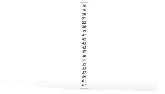
Next, each age value is tallied to create the frequency. This is an example of an ungrouped frequency distribution. In an ungrouped frequency distribution, researchers list all categories of the variable on which they have data and tally each datum on the listing. In this example, all the different ages of the 20 patients are listed and then tallied for each age.

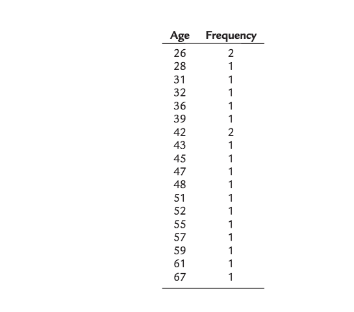
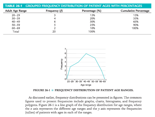
Because most of the ages in this dataset have frequencies of “1,” it is better to group the ages into ranges of values. These ranges must be mutually exclusive (i.e., a patient’ s age can only be classified into one of the ranges). In addition, the ranges must be exhaustive, meaning that each patient’ s age will fi t into at least one of the categories. For example, we may choose to have ranges of 10, so that the age ranges are 20 to 29, 30 to 39, 40 to 49, 50 to 59, and 60 to 69. We may choose to have ranges of 5, so that the age ranges are 20 to 24, 25 to 29, 30 to 34, etc. The grouping should be devised to provide the greatest possible meaning to the purpose of the study. If the data are to be compared with data in other studies, groupings should be similar to those of other studies in this field of research. Classifying data into groups results in the development of a grouped frequency distribution. Table 26-1 presents a grouped frequency distribution of patient ages classified by ranges of 10 years. Note that the range starts at “20” because there are no patient ages lower than 20, nor are there ages higher than 69. Table 26-1 also includes percentages of patients with an age in each range; the cumulative percentages for the sample should add up to 100%. This table provides an example of a percentage distribution that indicates the percentage of the sample with scores falling into a specific group. Percentage distributions are particularly useful in comparing this study’s data with results from other studies.

QUESTIONS

1. Plot the frequency distribution for “Age at Enrollment” by hand or by using SPSS.

2. How would you characterize the skewness of the distribution in Question 1—positively skewed, negatively skewed, or approximately normal? Provide a rationale for your answer.

3. Compare the original skewness statistic and Shapiro-Wilk statistic with those of the smaller dataset ( n = 15) for the variable “Age at First Arrest.” How did the statistics change, and how would you explain these differences?

4. Plot the frequency distribution for “Years of Education” by hand or by using SPSS.

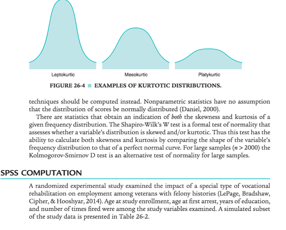
5. How would you characterize the kurtosis of the distribution in Question 4—leptokurtic, mesokurtic, or platykurtic? Provide a rationale for your answer.

6. What is the skewness statistic for “Age at Enrollment”? How would you characterize the mag-nitude of the skewness statistic for “Age at Enrollment”?

7. What is the kurtosis statistic for “Years of Education”? How would you characterize the magnitude of the kurtosis statistic for “Years of Education”?

8. Using SPSS, compute the Shapiro-Wilk statistic for “Number of Times Fired from Job.” What would you conclude from the results?

9. In the SPSS output table titled “Tests of Normality,” the Shapiro-Wilk statistic is reported along with the Kolmogorov-Smirnov statistic. Why is the Kolmogorov-Smirnov statistic inappropriate to report for these example data?

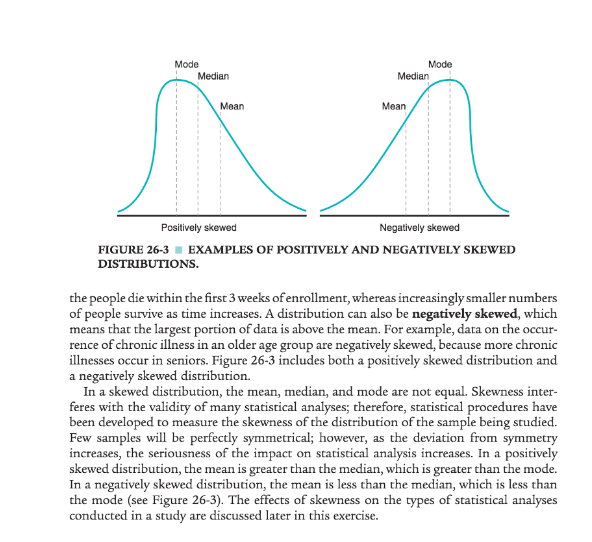
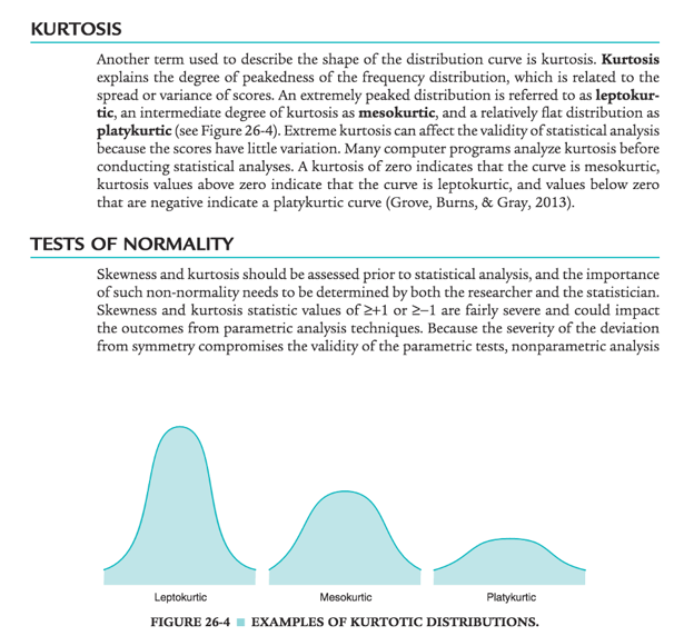
10. How would you explain the skewness statistic for a particular frequency distribution being low and the Shapiro-Wilk statistic still being significant at p < 0.05?